8.8 Order analysis on various schemes for the advection equation
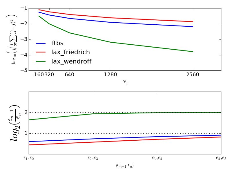
The schemes presented have different theoretical order; ftbs: \( \mathcal{O}\left(\Delta x, \Delta t\right) \), Lax-Friedrich: \( \mathcal{O}\left(\Delta x^2, \Delta t\right) \), Lax-Wendroff: \( \mathcal{O}\left(\Delta x^2, \Delta t^2\right) \), MacCormack: \( \mathcal{O}\left(\Delta x^2, \Delta t^2\right) \). For the linear advection equation the MacCormack and Lax-Wendroff schemes are identical, and we will thus only consider Lax-Wendroff in this section. Assuming the wavespeed \( a_0 \) is not very big, nor very small we will have \( \Delta t=\mathcal{O}\left(\Delta x\right) \), because of the cfl constraint condition. Thus for the advection schemes the discretization error \( \epsilon \) will be of order min(\( p, q \)). Where \( p \) is the spatial order, and \( q \) the temporal order. Thus we could say that ftbs, and Lax-Friedrich are both first order, and Lax-Wendroff is of second order. In order to determine the observed (dominating) order of accuracy of our schemes we could adapt the same procedure outlined in Example 2.8.1 Example: Numerical error as a function of \( \Delta t \), where we determined the observed order of accuracy of ODEschemes. For the schemes solving the Advection equation the discretization error will be a combination of \( \Delta x \) and \( \Delta t \), however since \( \Delta t=\mathcal{O}\left(\Delta x\right) \), we may still assume the following expression for the discretization error: $$ \begin{align} \tag{8.55} \epsilon \approx Ch^p \end{align} $$ where \( h \) is either \( \Delta x \) or \( \Delta t \), and \( p \) is the dominating order. Further we can calculate the discretization error, observed for our schemes by successively refining \( h \) with a ratio \( r \), keeping the cfl-number constant. Thus refining \( \Delta x \) and \( \Delta t \) with the same ratio \( r \). Now dividing \( \epsilon_{n-1} \) by \( \epsilon_{n} \) and taking the log on both sides and rearranging lead to the following expression for the observed order of accuracy: $$ \begin{align} p = \frac{log\left(\frac{{\epsilon}_{n-1}}{{\epsilon}_n} \right)}{log\left(r \right)} = log_r\left(\frac{\epsilon_{n-1}}{\epsilon_n} \right) \nonumber \end{align} $$ To determine the observed discretization error we will use the root mean square error of all our discrete solutions: $$ \begin{align} E = \sqrt{\frac{1}{N}\sum\limits_{i=1}^N\left(\hat{f}-f\right)^2} \nonumber \end{align} $$ where N is the number of sampling points, \( \hat f \) is the numerical-, and \( f \) is the analytical solution. A code example performing this test on selected advections schemes, is showed below. As can be seen in Figure 113, the Lax-Wendroff scheme quickly converge to it's theoretical order, whereas the ftbs and Lax Friedrich scheme converges to their theoretical order more slowly.
Figure 113: The root mean square error \( E \) for the various advection schemes as a function of the number of spatial nodes (top), and corresponding observed convergence rates (bottom).
    def test_convergence_MES():
        from numpy import log
        from math import sqrt
        global c, dt, dx, a

        # Change default values on plots
        LNWDT=2; FNT=13
        plt.rcParams['lines.linewidth'] = LNWDT; plt.rcParams['font.size'] = FNT

        a = 1.0 # wave speed
        tmin, tmax = 0.0, 1 # start and stop time of simulation
        xmin, xmax = 0.0, 2.0 # start and end of spatial domain
        Nx = 160 # number of spatial points
        c = 0.8 # courant number, need c<=1 for stability

        # Discretize
        x = np.linspace(xmin, xmax, Nx + 1) # discretization of space
        dx = float((xmax-xmin)/Nx) # spatial step size
        dt = c/a*dx # stable time step calculated from stability requirement
        time = np.arange(tmin, tmax + dt, dt) # discretization of time

        init_funcs = [init_step, init_sine4] # Select stair case function (0) or sin^4 function (1)
        f = init_funcs[1]

        solvers = [ftbs, lax_friedrich, lax_wendroff]

        errorDict = {} # empty dictionary to be filled in with lists of errors
        orderDict = {}

        for solver in solvers:
            errorDict[solver.__name__] = [] # for each  solver(key) assign it with value=[], an empty list (e.g: 'ftbs'=[])
            orderDict[solver.__name__] = []

        hx = [] # empty list of spatial step-length
        ht = [] # empty list of temporal step-length

        Ntds = 5 # number of grid/dt refinements
        # iterate Ntds times:
        for n in range(Ntds):
            hx.append(dx)
            ht.append(dt)

            for k, solver in enumerate(solvers): # Solve for all solvers in list
                u = f(x) # initial value of u is init_func(x)
                error = 0
                samplePoints = 0

                for i, t in enumerate(time[1:]):
                    u_bc = interpolate.interp1d(x[-2:], u[-2:]) # interplate at right bndry
                    u[1:-1] = solver(u[:]) # calculate numerical solution of interior
                    u[-1] = u_bc(x[-1] - a*dt) # interpolate along a characteristic to find the boundary value

                    error += np.sum((u - f(x-a*t))**2) # add error from this timestep
                    samplePoints += len(u)

                error = sqrt(error/samplePoints) # calculate rms-error
                errorDict[solver.__name__].append(error)

                if n>0:
                    previousError = errorDict[solver.__name__][n-1]
                    orderDict[solver.__name__].append(log(previousError/error)/log(2))

            print(" finished iteration {0} of {1}, dx = {2}, dt = {3}, tsample = {4}".format(n+1, Ntds, dx, dt, t))
            # refine grid and dt:
            Nx *= 2
            x = np.linspace(xmin, xmax, Nx+1) # new x-array, twice as big as the previous
            dx = float((xmax-xmin)/Nx) # new spatial step size, half the value of the previous
            dt = c/a*dx # new stable time step
            time = np.arange(tmin, tmax + dt, dt) # discretization of time

        # Plot error-values and corresponding order-estimates:
        fig , axarr = plt.subplots(2, 1, squeeze=False)
        lstyle = ['b', 'r', 'g', 'm']
        legendList = []

        N = Nx/2**(Ntds + 1)
        N_list = [N*2**i for i in range(1, Ntds+1)]
        N_list = np.asarray(N_list)

        epsilonN = [i for i in range(1, Ntds)]
        epsilonlist = ['$\epsilon_{0} , \epsilon_{1}$'.format(str(i), str(i+1)) for i in range(1, Ntds)]

        for k, solver in enumerate(solvers):
            axarr[0][0].plot(N_list, np.log10(np.asarray(errorDict[solver.__name__])),lstyle[k])
            axarr[1][0].plot(epsilonN, orderDict[solver.__name__],lstyle[k])

            legendList.append(solver.__name__)


        axarr[1][0].axhline(1.0, xmin=0, xmax=Ntds-2, linestyle=':', color='k')
        axarr[1][0].axhline(2.0, xmin=0, xmax=Ntds-2, linestyle=':', color='k')
8.8.1 Separating spatial and temporal discretization error
The test performed in the previous example verify the dominating order of accuracy of the advection schemes. However in order to verify our implementations of the various schemes we would like to ensure that both the observed temporal- and spatial order are close to the theoretical orders. The expression for the discretization error in (8.55) is a simplification of the more general expression $$ \begin{align} \tag{8.56} \epsilon \approx C_x \: h_x^p + C_t \: h_t^q \end{align} $$ where \( C_x \), and \( C_t \) are constants, \( h_x \) and \( h_t \) are the spatial- and temporal step lengths and \( p \) and \( q \) are the spatial- and temporal orders respectively. We are interested in confirming that \( p \) is close to the theoretical spatial order of the scheme, and that \( q \) is close to the theoretical temporal order of the scheme. The method of doing this is not necessarily straight forward, especially since \( h_t \) and \( h_x \) are coupled through the cfl-constraint condition. In chapter one we showed that we were able to verify \( C \) and \( p \) in the case of only one step-length dependency (time or space), by solving two nonlinear equations for two unknowns using a Newton-Rhapson solver. To expand this method would now involve solving four nonlinear algebraic equations for the four unknowns \( C_x, C_t, p, q \). However since it is unlikely that the observed discretization error match the expression in (8.56) exactly, we now suggest a method based on optimization and curve-fitting. From the previous code example we calculated the root mean square error \( E(h_x, h_t) \) of the schemes by successively refining \( hx \) and \( ht \) by a ratio \( r \). We now assume that \( E \) is related to \( C_x, C_t, p, q \) as in (8.56). In other words we would like to find the parameters \( C_x, C_t, p, q \), so that the difference between our calculated errors \( E(hx, ht) \), and the function \( \epsilon\left(h_x, h_t;C_x, p, C_t, q\right) = C_x \: h_x^p + C_t \: h_t^q \) is as small as possible. This may be done by minimizing the sum (\( S \)) of squared residuals of \( E \) and \( \epsilon \): $$ \begin{align} S = \sum\limits_{i=1}^N r_i^2, \quad r_i= E_i - \epsilon\left(h_x, h_t;C_x, p, C_t, q\right)_i \nonumber \end{align} $$ The python module scipy.optimize has many methods for parameter optimization and curve-fitting. In the code example below we use scipy.optimize.curve_fit which fits a function "f(x;params)" to a set of data "y-data" using a Levenberg-Marquardt algorithm with a least square minimization criteria. In the code example below we start by loading the calculated root mean square errors \( E\left(h_{x}, h_{t}\right) \) of the schemes from "advection_scheme_errors.txt", which where calculated in the same manner as in the previous example. As can be seen by Figure 113 the ftbs, and Lax Friedriech scheme takes a while before they are in their asymptotic range (area where they converge at a constant rate). In "advection_scheme_errors.txt" we have computed \( E\left(h_{x}, h_{t}\right) \) up to \( N_x = 89120 \) in which all schemes should be close to their asymptotic range. This procedure is demonstrated in the code example below in which the following expressions for the errors are obtained: $$ \begin{align} \tag{8.57} ftbs \rightarrow \epsilon = 1.3 \: h_x^{0.98} + 6.5 \: h_t^{0.98} \\ lax Friedrich \rightarrow \epsilon = - 1484 \: h_x^{1.9} + 26 \: h_t^{1.0} \tag{8.58}\\ lax Wendroff \rightarrow \epsilon = - 148 \: h_x^{2.0} + 364. \: h_t^{2.0} \tag{8.59} \end{align} $$
import numpy as np
import matplotlib.pyplot as plt
from scipy.optimize import curve_fit
from sympy import symbols, lambdify, latex

def optimize_error_cxct(errorList, hxList,
                        htList, p=1.0, q=1.0):
    """ Function that optimimze the values Cx and Ct in the expression
        E = epsilon = Cx hx^p + Ct ht^q, assuming p and q are known,
        using scipy's optimization tool curve_fit

        Args:
            errorList(array): array of calculated numerical discretization errors E
            hxList(array): array of spatial step lengths corresponding to errorList
            htList(array): array of temporal step lengths corresponding to errorList
            p (Optional[float]): spatial order. Assumed to be equal to theoretical value
            q (Optional[float]): temporal order. Assumed to be equal to theoretical value

        Returns:
            Cx0(float): the optimized values of Cx
            Ct0(float): the optimized values of Ct
    """

    def func(h, Cx, Ct):
        """ function to be matched with ydata:
            The function has to be on the form func(x, parameter1, parameter2,...,parametern)
            where where x is the independent variable(s), and parameter1-n are the parameters to be optimized.
        """
        return Cx*h[0]**p + Ct*h[1]**q


    x0 = np.array([1,2]) # initial guessed values for Cx and Ct
    xdata = np.array([hxList, htList])# independent variables
    ydata = errorList # data to be matched with expression in func
    Cx0, Ct0 = curve_fit(func, xdata, ydata, x0)[0] # call scipy optimization tool curvefit

    return Cx0, Ct0

def optimize_error(errorList, hxList, htList,
                   Cx0, p0, Ct0, q0):
    """ Function that optimimze the values Cx, p Ct and q in the expression
        E = epsilon = Cx hx^p + Ct ht^q, assuming p and q are known,
        using scipy's optimization tool curve_fit

        Args:
            errorList(array): array of calculated numerical discretization errors E
            hxList(array): array of spatial step lengths corresponding to errorList
            htList(array): array of temporal step lengths corresponding to errorList
            Cx0 (float): initial guessed value of Cx
            p (float): initial guessed value of p
            Ct0 (float): initial guessed value of Ct
            q (float): initial guessed value of q

        Returns:
            Cx(float): the optimized values of Cx
            p (float): the optimized values of p
            Ct(float): the optimized values of Ct
            q (float): the optimized values of q
    """


    def func(h, gx, p, gt, q):
        """ function to be matched with ydata:
            The function has to be on the form func(x, parameter1, parameter2,...,parametern)
            where where x is the independent variable(s), and parameter1-n are the parameters to be optimized.
        """
        return gx*h[0]**p + gt*h[1]**q


    x0 = np.array([Cx0, p0, Ct0, q0]) # initial guessed values for Cx, p, Ct and q
    xdata = np.array([hxList, htList]) # independent variables
    ydata = errorList # data to be matched with expression in func

    gx, p, gt, q = curve_fit(func, xdata, ydata, x0)[0] # call scipy optimization tool curvefit
    gx, p, gt, q = round(gx,2), round(p, 2), round(gt,2), round(q, 2)

    return gx, p, gt, q

# Program starts here:

# empty lists, to be filled in with values from 'advection_scheme_errors.txt'
hxList = []
htList = []

E_ftbs = []
E_lax_friedrich = []
E_lax_wendroff = []

lineNumber = 1

with open('advection_scheme_errors.txt', 'r') as FILENAME:
    """ Open advection_scheme_errors.txt for reading.
        structure of file:
        hx    ht    E_ftbs    E_lax_friedrich    E_lax_wendroff

        with the first line containing these headers, and the next lines containing
        the corresponding values.
    """
    # iterate all lines in FILENAME:
    for line in FILENAME:
        if lineNumber ==1:
            # skip first line which contain headers
            lineNumber += 1
        else:
            lineList = line.split() # sort each line in a list: lineList = [hx, ht, E_ftbs, E_lax_friedrich, E_lax_wendroff]

            # add values from this line to the lists
            hxList.append(float(lineList[0]))
            htList.append(float(lineList[1]))

            E_ftbs.append(float(lineList[2]))
            E_lax_friedrich.append(float(lineList[3]))
            E_lax_wendroff.append(float(lineList[4]))

            lineNumber += 1

FILENAME.close()

# convert lists to numpy arrays:
hxList = np.asarray(hxList)
htList = np.asarray(htList)


E_ftbs = np.asarray(E_ftbs)
E_lax_friedrich = np.asarray(E_lax_friedrich)
E_lax_wendroff = np.asarray(E_lax_wendroff)


ErrorList = [E_ftbs, E_lax_friedrich, E_lax_wendroff]
schemes = ['ftbs', 'lax_friedrich', 'lax_wendroff']

p_theoretical = [1, 2, 2] # theoretical spatial orders
q_theoretical = [1, 1, 2] # theoretical temporal orders

h_x, h_t = symbols('h_x h_t')

XtickList = [i for i in range(1, len(hxList)+1)]
Xticknames = [r'$(h_x , h_t)_{0}$'.format(str(i)) for i in range(1, len(hxList)+1)]
lstyle = ['b', 'r', 'g', 'm']
legendList = []

# Optimize Cx, p, Ct, q for every scheme
for k, E in enumerate(ErrorList):

    # optimize using only last 5 values of E and h for the scheme, as the first values may be outside asymptotic range:

    Cx0, Ct0 = optimize_error_cxct(E[-5:], hxList[-5:], htList[-5:],
                                   p=p_theoretical[k], q=q_theoretical[k]) # Find appropriate initial guesses for Cx and Ct

    Cx, p, Ct, q = optimize_error(E[-5:], hxList[-5:], htList[-5:],
                                  Cx0, p_theoretical[k], Ct0, q_theoretical[k]) # Optimize for all parameters Cx, p, Ct, q

    # create sympy expressions of e, ex and et:
    errorExpr = Cx*h_x**p + Ct*h_t**q

    print(errorExpr)
    errorExprHx = Cx*h_x**p
    errorExprHt = Ct*h_t**q

    # convert e, ex and et to python functions:
    errorFunc = lambdify([h_x, h_t], errorExpr)
    errorFuncHx = lambdify([h_x], errorExprHx)
    errorFuncHt = lambdify([h_t], errorExprHt)

    # plotting:
    fig , ax = plt.subplots(2, 1, squeeze=False)

    ax[0][0].plot(XtickList, np.log10(E),lstyle[k])
    ax[0][0].plot(XtickList, np.log10(errorFunc(hxList, htList)),lstyle[k] + '--')

    ax[1][0].plot(XtickList[-5:], E[-5:],lstyle[k])
    ax[1][0].plot(XtickList[-5:], errorFunc(hxList, htList)[-5:],lstyle[k] + '--')
    ax[1][0].plot(XtickList[-5:], errorFuncHx(hxList[-5:]), lstyle[k] + '-.')
    ax[1][0].plot(XtickList[-5:], errorFuncHt(htList[-5:]),lstyle[k] + ':')
Figure 114: Optimized error expressions for all schemes. Test using doconce combine images
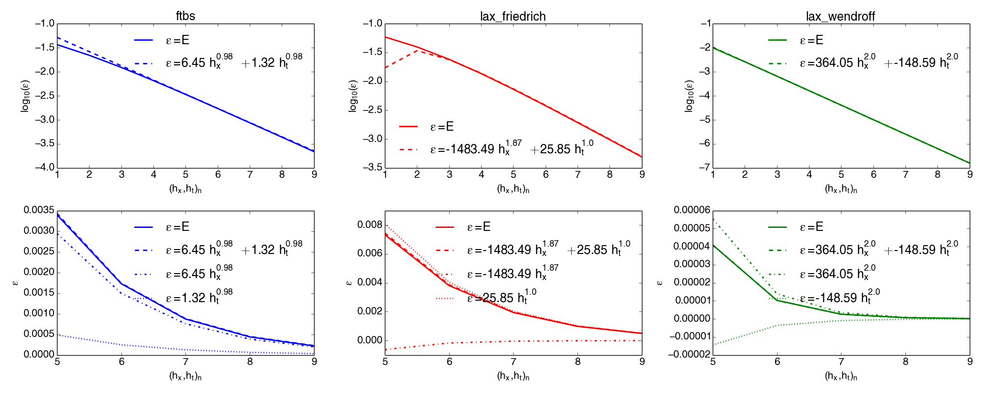
Figure 115: The solutions at time t=T=1 for different grids corresponding to the code-example above. A \( sin^4 \) wave with period \( T= 0.4 \) travelling with wavespeed \( a \) = 1. The solutions were calculated with a cfl-number of 0.8
