2.15 Absolute stability of numerical methods for ODE IVPs
To investigate stability of numerical methods for the solution of intital value ODEs on the generic form (2.2), let us consider the following model problem: $$ \begin{align} y'(x) & =\lambda \cdot y(x) \tag{2.129} \\ y(0)& =1 \tag{2.130} \end{align} $$ which has the analytical solution: $$ \begin{equation} y(x)=e^{\lambda x},\ \lambda\,, \tag{2.131} \end{equation} $$ with \( \lambda \) being a constant.
The solution \( y(x) \) of (2.129) is illustrated in Figure 22 for positive (\( \lambda = 1 \)) and negative (\( \lambda = -2 \)) growth factors.
Figure 22: Solution of ODE for exponential growth with positive and negative growth factor \( \lambda \).

We illustrate the stability concept for the numerical solution of ODEs by two examples below, namely, the Euler scheme and the Heun scheme. In the latter example we will also allude to how the analysis may be applied for higher order RK-methods.
2.15.1 Example: Stability of Euler's method
By applying the generic 2.6 Euler's method On our particular model problem given by (2.129) we obtain the following generic scheme: $$ \begin{equation} y_{n+1}= (1+\lambda h)\, y_n,\qquad h=\Delta x,\quad n=0,1,2,\dots \tag{2.132} \end{equation} $$
The numerical soltion \( y_n \) at the \( n \)-th iteration may be related with the initial solution \( y_0 \) by applying the scheme (2.132) iteratively: $$ \begin{align*} y_1&=(1+\lambda h)\, y_0\\ y_2&=(1+\lambda h)\, y_1=(1+\lambda h)^2\, y_0\\ &\vdots & \end{align*} $$ which yields: $$ \begin{equation} y_n=(1+\lambda h)^n\, y_0, \qquad n=1,2,3,\dots \tag{2.133} \end{equation} $$
To investigate stability we first introduce the analytic amplification factor \( G_a \) as $$ \begin{equation} G_a=\frac{y(x_{n+1})}{y(x_n)} \tag{2.134} \end{equation} $$
Note that \( y(x_n) \) represents the analytical solution of (2.129) at \( x_n \), whereas \( y_n \) denotes the numerical approximation. For the model problem at hand we see that \( G_a \) reduces to: $$ \begin{equation} G_a=\frac{y(x_{n+1})}{y(x_n)}=\exp[\lambda (x_{n+1}-x_n)]=e^{\lambda h}=1 + \lambda h +(\lambda h)^2/2 \dots \tag{2.135} \end{equation} $$
Exponential growth \( \lambda > 0 \).
Consider first the case of a positive \( \lambda > 0 \), corresponding to an exponential growth, as given by (2.131). We observe that our scheme will also exhibit exponential growth (2.134), and will thus have no concerns in terms of stability. Naturally, the choice of \( h \) will affect the accuracy and numerical error of the solution.
Exponential decay \( \lambda < 0 \).
In case of exponential decay with a negative \( \lambda < 0 \), we adopt the following convention for convenience: $$ \begin{equation} \lambda = -\alpha, \qquad \alpha > 0 \tag{2.136} \end{equation} $$
and (2.133) may be recasted to: $$ \begin{equation} y_n=(1-\alpha h)^n\, y_0 \tag{2.137} \end{equation} $$
If \( y_n \) is to decrease as \( n \) increases we must have $$ \begin{equation} |1-\alpha h| < 1 \qquad \Rightarrow -1 < 1-\alpha h < 1 \tag{2.138} \end{equation} $$ which yields the following criterion for selection of \( h \): $$ \begin{equation} \tag{2.139} 0 < \alpha h < 2,\ \alpha > 0 \end{equation} $$
The criterion may also be formulated by introducing the numerical amplification factor \( G \) as: $$ \begin{align} G= & \frac{y_{n+1}}{y_n} \tag{2.140} \end{align} $$ which for the current example (2.132) reduces to: $$ \begin{align} G & = \frac{y_{n+1}}{y_n}=1+\lambda h = 1-\alpha h \tag{2.141} \end{align} $$ For the current example \( G > 1 \) for \( \lambda > 0 \) and \( G < 1 \) for \( \lambda < 0 \). Compare with the expression for the analytical amplification factor \( G_a \) (2.135).
As we shall see later on, the numerical amplification factor \( G(z) \) is some function of \( z=h\lambda \), commonly a polynomial for an explicit method and a rational function for implicit methods. For consistent methods \( G(z) \) will be an approximation to \( e^z \) near \( z=0 \), and if the method is \( p \)-th order accurate, then \( G(z)-e^z= \mathcal{O}(z^{p+1}) \) as \( z \to 0 \).
For example, in the case under examination, when \( \alpha=100 \) we must choose \( h < 0.02 \) to produce an stable numerical solution.
By the introduction of the \( G \) in (2.141) we may rewrite (2.133) as: $$ \begin{equation} \tag{2.145} y_n=G^n\, y_0,\qquad n=0,1,2,\dots \end{equation} $$
From (2.145) we observe that a stable, exponentially decaying solution (\( \lambda < 0 \) ) the solution will oscillate if \( G < 0 \), as \( G^n < 0 \) when \( n \) is odd and \( G^n > 0 \) when \( n \) is even. As this behavior is qualitatively different from the behaviour of the analytical solution, we will seek to avoid such behavior.
The Euler scheme is conditionally stable for our model equation when $$ \begin{align} 0 < \alpha h < 2,\ \alpha > 0 \tag{2.146} \end{align} $$
but oscillations will occur when $$ \begin{align} 1 < \alpha h < 2,\ \alpha >0 \tag{2.147} \end{align} $$
Consequently, the Euler scheme will be stable and free of spurious oscillations when $$ \begin{align} 0 < \alpha h < 1, \qquad \alpha > 0 \tag{2.148} \end{align} $$
For example the numerical solution with \( \alpha =10 \) will be stable in the intervall \( 0 < h < 0 .2 \), but exhibit oscillations in the interval \( 0.1 < h < 0.2 \). Note, however, that the latter restriction on avoiding spurious oscillations will not be of major concerns in pratice, as the demand for descent accuracy will dictate a far smaller \( h \).
2.15.2 Example: Stability of Heun's method
In this example we will analyze the stability of 2.9 Heun's method when applied on our model ODE (2.129) with \( \lambda = -\alpha,\ \alpha>0 \).
The predictor step reduces to: $$ \begin{align} y^p_{n+1} & = y_n +h\cdot f_n=(1-\alpha h) \cdot y_n \tag{2.149} \end{align} $$
for convenience the predictor \( y^p_{n+1} \) may be eliminated in the corrector step: $$ \begin{align} y_{n+1} & =y_n+\frac{h}{2} \cdot (f_n+f^p_{n+1})= (1-\alpha h+\frac{1}{2}(\alpha h)^2) \cdot y_n \tag{2.150} \end{align} $$
which shows that Heun's method may be represented as a one-step method for this particular and simple model problem. From (2.150) we find the numerical amplification factor \( G \) (ref<{eq:1618a}); $$ \begin{equation} G=\frac{y_{n+1}}{y_n}=1-\alpha h+\frac{1}{2}(\alpha h)^2 \tag{2.151} \end{equation} $$
Our taks is now to investigate for which values of \( \alpha h \) the condition for stability (2.143) may be satisfied.
First, we may realize that (2.151) is a second order polynomial in \( \alpha h \) and that \( G=1 \) for \( \alpha h =0 \) and \( \alpha h = 2 \). The numerical amplification factor has an extremum where: $$ \begin{equation*} \frac{dG}{d \alpha h}= \alpha h -1 = 0 \Rightarrow \alpha h = 1 \end{equation*} $$ and since $$ \begin{equation*} \frac{d^2G}{d (\alpha h)^2} > 0 \end{equation*} $$ this extremum is a minimum and \( G_{\min}=G(\alpha h=1)= 1/2 \). Consequently we may conclude that 2.9 Heun's method will be conditionally stable for (2.129) in the following \( \alpha h \)-range (stability range): $$ \begin{equation} 0 < \alpha h < 2 \tag{2.152} \end{equation} $$
Note that this condition is the same as for the 2.15.1 Example: Stability of Euler's method above, but as \( G > 0 \) always, the scheme will not produce spurious oscillations.
The 2.6 Euler's method and 2.9 Heun's method are RK-methods of first and second order, respectively. Even though the \( \alpha h \)-range was not expanded by using a RK-method of 2 order, the quality of the numerical predictions were improved as spurios oscillations will vanish.
2.15.3 Stability of higher order RK-methods
A natural questions to raise is whether the stability range may be expanded for higher order RK-methods, so let us now investigate their the stability range.
The analytical solution of our model ODE (2.129) is: $$ \begin{equation} \tag{2.153} y(x)=e^{\lambda x}=1+\lambda x +\frac{(\lambda x)^2}{2!}+\frac{(\lambda x)^3}{3!}+\cdots+\frac{(\lambda x)^n}{n!}+\cdots \end{equation} $$
By substitution of \( \lambda x \) with \( \lambda h \), we get the solution of the difference equation corresponding to Euler's method (RK1) with the two first terms, Heun's method (RK2) the three first terms RK3 the four first terms, and finally RK4 with the first five terms: $$ \begin{equation} G=1+\lambda h +\frac{(\lambda h)^2}{2!}+\frac{(\lambda h)^3}{3!}+\cdots+\frac{(\lambda h)^n}{n!}. \tag{2.154} \end{equation} $$
We focus on decaying solutions with \( \lambda < 0 \) and we have previously show from (2.139) that \( 0 < \alpha h < 2,\alpha > 2 \) or: $$ \begin{equation} -2 < \lambda h < 0 \tag{2.155} \end{equation} $$ for RK1 and RK3, but what about RK3? In this case: $$ \begin{equation} G=1+\lambda h + \frac{(\lambda h)^2}{2!}+\frac{(\lambda h)^3}{3!} \tag{2.156} \end{equation} $$
The limiting values for the \( G \)-polynomial are found for \( G = \pm1 \) which for real roots are: $$ \begin{equation} -2.5127 < \lambda h < 0 \tag{2.157} \end{equation} $$
For RK4 we get correspondingly $$ \begin{equation} G =1+\lambda h + \frac{(\lambda h)^2}{2!}+\frac{(\lambda h)^3}{3!}+\frac{(\lambda h)^4}{4!} \tag{2.158} \end{equation} $$
which for \( G=1 \) has the real roots: $$ \begin{equation} -2.7853 < \lambda h < 0 \tag{2.159} \end{equation} $$
In conclusion, we may argue that with respect to stability there is not much to gain by increasing the order for RK-methods. We have assumed \( \lambda \) to be real in the above analysis. However, \( \lambda \) may me complex for higer order ODEs and for systems of first order ODEs. If complex roots are included the regions of stability for RK-methods become as illstrated in figure 23.
Figure 23: Regions of stability for RK-methods order 1-4 for complex roots.
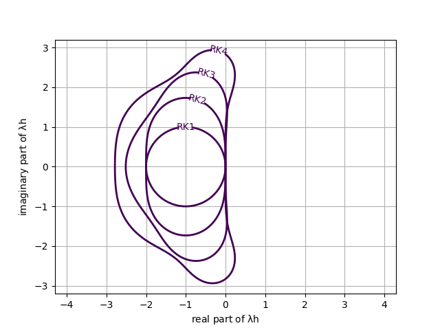
Naturally, we want numerical schemes which are stable in the whole left half-plane. Such a scheme would be denoted strictly absolutely stable or simply L-stable (where L alludes to left half-plane). Regretfully, there are no existing, explicit methods which are L-stable. For L-stable methods one has to restort to implicit methods which are to be discussed in 2.15.4 Stiff equations.
2.15.4 Stiff equations
While there is no precise definition of stiff ODEs in the literature, these are some generic characteristics for ODEs/ODE systems that are often called as such:
- ODE solution has different time scales. For example, the ODE solution can be written as the sum of a fast and a slow component as:
- For a first ODE system
the above statement is equivalent to the case in which the eigenvalues of the Jacobian \( \frac{\partial \boldsymbol{f}}{\partial \boldsymbol{y}} \) differ greatly in magnitude.
- The definition of \( h \) for stiff ODEs is limited by stability concerns rather than by accuracy.
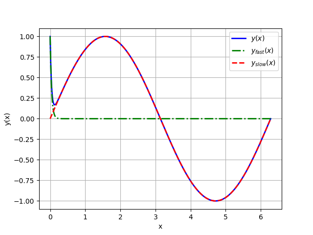
Example for stiff ODE: Consider the IVP $$ \begin{equation} \left. \begin{aligned} & y' = \lambda y - \lambda sin(x) + cos(x), \quad\quad \lambda < 0,\\ & y(0) = 1. \end{aligned} \right\} \end{equation}\tag{2.160} $$
The analytical solution of problem (2.160) is given by $$ \begin{equation*} y(x) = sin(x) + e^{\lambda x}, \tag{2.161} \end{equation*} $$
from which we can identify a slow component $$ \begin{equation*} y_{slow}(x) = sin(x) \end{equation*} $$
and a fast component $$ \begin{equation*} y_{fast}(x) = e^{\lambda x}, \end{equation*} $$
for \( |\lambda| \) sufficiently large.
Figure 24: Solution (2.161) of stiff ODE IVP (2.160) for \( \lambda=-25 \).
A way to avoid having to use excessively small time steps, which can be even harmful for the accuracy of the approximation, due to error accumulation, is to use numerical schemes which have a larger region of absolute stability than explicit schemes.
2.15.5 Example: Stability of implicit Euler's method
The most natural, and widely used, candidate as a replacement of an explicit first order scheme is the implicit Euler's scheme. Equation (2.129) discretized using this scheme reads $$ \begin{equation*} y_{n+1} = y_n + h f_{n+1} = y_n + h \lambda y_{n+1}, \end{equation*} \tag{2.162} $$
and after solving for \( y_{n+1} \) $$ \begin{equation*} y_{n+1} = \frac{1}{1- h \lambda} y_n. \end{equation*} $$
Therefore, the amplification factor for this scheme is $$ \begin{equation*} G = \frac{1}{1- h \lambda} = \frac{1}{1 + h \alpha}, \quad \lambda = - \alpha,\quad \alpha > 0. \end{equation*} $$
It is evident that \( G < 1 \) for any \( h \) (recall that \( h \) is positive by definition). This means that the interval of absolute stability for the implicit Euler's scheme includes \( \mathbb{R}^- \). If this analysis was carried out allowing for \( \lambda \) to be a complex number with negative real part, then the region of absolute stability for the implicit Euler's scheme would have included the entire complex half-plane with negative real part \( \mathbb{C}^- \).
2.15.6 Example: Stability of trapezoidal rule method
Equation (2.129) discretized by the trapezoidal rule scheme reads $$ \begin{equation*} y_{n+1} = y_n + \frac{h}{2} (f_n + f_{n+1}) = y_n + \frac{h}{2} (\lambda y_n + \lambda y_{n+1}), \end{equation*} \tag{2.163} $$
and after solving for \( y_{n+1} \) $$ \begin{equation*} y_{n+1} = \frac{1+\frac{\lambda h}{2}}{1-\frac{\lambda h}{2}} y_n. \end{equation*} $$
Therefore, the amplification factor for this scheme is $$ \begin{equation*} G = \frac{1+\frac{\lambda h}{2}}{1-\frac{\lambda h}{2}} = \frac{2 - \alpha h}{2 + \alpha h}, \quad \lambda = - \alpha,\quad \alpha > 0. \end{equation*} $$
As for the implicit Euler's scheme, also in this case we have that \( G < 1 \) for any \( h \). Therefore, interval of absolute stability for the implicit Euler's scheme includes \( \mathbb{R}^- \). In this case, the analysis for \( \lambda \) complex number with negative real part, would have shown that the region of absolute stability for this scheme is precisely the entire complex half-plane with negative real part \( \mathbb{C}^- \).
The above results motivate the following definition:
This important definition was introduced in the '60s by Dahlquist, who also proved that A-stable schemes can be most second order accurate. A-stable schemes are unconditionally stable and therefore robust, since no stability problems will be observed. However, the user must always be aware of the fact that even if one is allowed to take a large value for \( h \), the error must be contained within acceptable limits.