7.7 Example with radial symmetry
If we write the diffusion equation \( \frac{\partial u}{\partial t}=\frac{\partial^2 u}{\partial x^2}+\frac{\partial^2 u}{\partial y^2}+\frac{\partial^2 u}{\partial z^2} \) for cylindrical and spherical coordinates and require \( u \) to be only a function of time \( t \) and radius \( r \), we have that:
Cylinder: $$ \begin{equation*} \frac{\partial u}{\partial t}= \frac{\partial^2 u}{\partial r^2}+\frac{1}{r}\frac{\partial u }{\partial r} \end{equation*} $$
Sphere: $$ \begin{equation*} \frac{\partial u}{\partial t}= \frac{\partial^2 u}{\partial r^2}+\frac{2}{r}\frac{\partial u }{\partial r} \end{equation*} $$
Both equations can be written as: $$ \begin{equation} \tag{7.91} \frac{\partial u}{\partial t}= \frac{\partial^2 u}{\partial r^2}+\frac{\lambda}{r}\frac{\partial u }{\partial r},\ \lambda=0,1,2 \end{equation} $$
\( \lambda=0 \) with \( r\to x \) gives the well-known Cartesian case.
(7.91) is a partial differential equation with variable coefficients. We will now perform a von Neumann stability analysis for this equation for the \( \theta \)-scheme from Section (7.5.3 Crank-Nicolson scheme. \( \theta \)-scheme).
Stability analysis using \( \theta \) -scheme for radius \( r > 0 \)
Setting \( r_j=\Delta r\cdot j,\ j=0,1,\dots \) and introducing \( D=\frac{\Delta t}{(\Delta r)^2} \)
For \( r > 0 \): $$ \begin{equation} \tag{7.92} \begin{array}{ll} u^{n+1}_j= &u^n_j+D\left[\theta(u^{n+1}_{j+1}-2u_j^{n+1}+u^{n+1}_{j-1})+(1-\theta)(u^n_{j+1}-2u^n_j+u^n_{j-1})\right]\\ \\ &+\frac{\lambda D}{2j} \left[\theta(u^{n+1}_{j+1}-u^{n+1}_{j-1})+(1-\theta)(u^n_{j+1}-u^n_{j-1}) \right] \end{array} \end{equation} $$
We proceed with the von Neumann analysis by inserting \( E^n_j=G^n\cdot e^{i\cdot \beta r_j}=G^ne^{i\cdot \delta\cdot j } \) with \( \delta=\beta\cdot \Delta r \) and using the usual formulas (7.50) and (7.51).
We get: $$ \begin{equation*} G\cdot \left( 1+4\theta D\sin^2\Big(\frac{\delta}{2}\Big)-i\cdot \frac{\theta\lambda D}{j}\sin(\delta)\right)=1-4(1-\theta)D\cdot \sin^2\Big(\frac{\delta}{2}\Big) +i \frac{(1-\theta)\lambda D}{j}\sin(\delta) \end{equation*} $$
which, using the formula \( \sin(\delta)=2\sin\Big(\dfrac{\delta}{2}\Big)\cos\Big(\dfrac{\delta}{2}\Big) \) and the condition \( |G|\leq1 \), becomes: $$ \begin{equation*} \left( 1-4(1-\theta) D\sin^2\Big(\frac{\delta}{2}\Big)\right)^2+\frac{(1-\theta)^2\lambda^2D^2}{j^2}\sin^2(\delta)\leq \left(1+4\theta D\sin^2\Big(\frac{\delta}{2}\Big) \right)^2 +\frac{\theta^2\lambda^2D^2}{j^2}\sin^2(\delta) \end{equation*} $$
and which further provides: $$ \begin{equation} \tag{7.93} D\cdot(1-2\theta)\cdot \left( \sin^2\Big(\frac{\delta}{2}\Big)\cdot\Big(4-\frac{\lambda^2}{j^2}\Big)+\frac{\lambda^2}{j^2} \right)\leq 2,\ j\geq1 \end{equation} $$
It is not difficult to see that the term in parenthesis has its largest value for \( \sin^2\Big(\dfrac{\delta}{2}\Big)=1 \); i.e. for \( \delta = \pi \). (This can also be found by deriving the term with respect to \( \delta \), which has its maximum for \( \delta = \pi \)). Factors \( \dfrac{\lambda^2}{j^2} \) fall then out.
We get: $$ \begin{equation} \tag{7.94} D\cdot (1-2\theta)\cdot 2\leq 1 \end{equation} $$
As in the section 7.5.3 Crank-Nicolson scheme. \( \theta \)-scheme, we must distinguish between two cases:
1. $$ \begin{equation*} 0\leq \theta \leq \frac{1}{2} \end{equation*} $$ $$ \begin{equation} \tag{7.95} D= \frac{\Delta t}{(\Delta r)^2} \leq \frac{1}{2(1-2\theta)} \end{equation} $$
2. $$ \begin{equation*} \frac{1}{2}\leq \theta \leq 1 \end{equation*} $$
Next we multiply (7.94) by \( -1 \): $$ \begin{equation*} D\cdot (2\theta-1)\cdot 2 \geq -1 \end{equation*} $$
This condition is always satisfied for the specified range of \( \theta \), so that in such cases the scheme is unconditionally stable.
In other words, we have obtain the same stability condition as for the equation with constant coefficients: \( \dfrac{\partial u}{\partial t}=\dfrac{\partial^2u}{\partial r^2} \), where we have the FTCS scheme for \( \theta=0 \), the Crank-Nicolson scheme for \( \theta=1/2 \), and the Laasonen scheme for \( \theta=1 \).
Note that this analysis is only valid for \( r > 0 \).
We now have a look at the equation for \( r=0 \).
The term \( \dfrac{\lambda}{r}\dfrac{\partial u}{\partial r} \) must be treated with special care for \( r=0 \).
L'Hopital's rule: $$ \begin{equation} \tag{7.96} \lim_{r\to 0}\frac{\lambda}{r}\frac{\partial u}{\partial r} = \lambda \frac{\partial^2u}{\partial r^2}\to \frac{\partial u}{\partial t}= (1+\lambda)\frac{\partial^2u}{\partial r^2} \text{ for }r=0 \end{equation} $$
We have found that using the FTCS scheme requires the usual constrain \( D\leq 1/2 \). Now we will check if boundary conditions pose some constrains when using the FTCS scheme.
Version 1
Discretize (7.96) for \( r=0 \) and use the symmetry condition \( \frac{\partial u}{\partial r}(0)=0 \): $$ \begin{equation} \tag{7.97} u^{n+1}_0=[1-2(1+\lambda)D]\cdot u_0^n+2(1+\lambda)D\cdot u^n_1 \end{equation} $$
If we use the PC-criterion on (7.97), we get: $$ \begin{equation} \tag{7.98} D\leq \frac{1}{2(1+\lambda)} \end{equation} $$
For \( \lambda = 0 \) we get the well-known condition \( D\leq 1/2 \), whereas for the cylinder (\( \lambda=1 \)) we get \( D\leq 1/4 \) and for the sphere, (\( \lambda =2 \)) we have \( D\leq 1/6 \). The question to be answered now is whether this conditions are for cylinder and sphere are necessary. We know that \( D\leq 1/2 \) is necessary and sufficient for \( \lambda=0 \).
It is difficult to find a necessary and sufficient condition in this case. Therefore, we concentrate in a special case: flow start-up in a tube, which is described in Example 7.7.1 Example: Start-up flow in a tube.
Version 2
To avoid using a separate equation for \( r=0 \) , we discretize \( \dfrac{\partial u}{\partial r}(0)=0 \) with a second order forward difference: $$ \begin{equation} \tag{7.99} \frac{\partial u }{\partial r}(0)=0\to \frac{-3u_0^n+4u^n_1-u_2^n}{2\Delta r}\to u^n_0=\frac{1}{3}(4u_1^n-u_2^n) \end{equation} $$
For a sphere, there is a detailed analysis by Dennis Eisen in the Journal Numerische Mathematik vol. 10, 1967, pages 397-409. The author shows that a necessary and sufficient condition for the solution of (7.92), along with (7.97) (for \( \lambda = 2 \) and \( \theta = 0 \)) is that \( D < 1/3 \). In addition, he shows that by avoiding the use of (7.97), the stability constrain for the FTCS scheme results to be \( D < 1/2 \).
Next we will go through two cases to see which stability requirements are obtained when one uses the two types of boundary conditions.
7.7.1 Example: Start-up flow in a tube
Figure 98: Velocity profile in a pipe at a given time.

Figure 98 shows the velocity profile of an incompressible fluid in a tube at a given time. The profile has reached the current configuration after evolving from a static configuration (velocity equal to 0 over the entire domain) by the application of a constant pressure gradient \( \frac{dp}{dz} < 0 \), so that we also know the velocity profile for the steady state configuration, which is the well-known parabolic profile for Poiseuille flow.
Under the above mentioned conditions, the momentum equation reads: $$ \begin{equation} \tag{7.100} \frac{\partial U}{\partial \tau}= -\frac{1}{\rho}\frac{dp}{dz}+\nu \left( \frac{\partial^2 U}{\partial R^2}+\frac{1}{R}\frac{\partial U}{\partial R} \right) \end{equation} $$
with \( U=U(R,\ \tau).\ 0\leq R \leq R_0, \) being the velocity profile and \( \tau \) the physical time.
Non-dimensional variables are: $$ \begin{equation} \tag{7.101} t=\nu \frac{\tau}{R^2_0},\ r= \frac{R}{R_0},\ u = \frac{U}{k},\ u_s= \frac{U_s}{k} \text{ der } k=-\frac{R_0^2}{4\mu}\frac{dp}{dz} \end{equation} $$
which introduced in (7.100) yield: $$ \begin{equation} \tag{7.102} \frac{\partial u}{\partial t }=4+ \frac{\partial^2u}{\partial r^2}+ \frac{1}{r}\frac{\partial u}{\partial r} \end{equation} $$
Boundary conditions are: $$ \begin{equation} \tag{7.103} u(\pm1,t)=0,\ \frac{\partial u}{\partial r}(0,t)=0 \end{equation} $$
The later is a symmetry condition. Finding a stationary solution requires that \( \frac{\partial u}{\partial t}=0 \): $$ \begin{equation*} \frac{d^2u_s}{dr^2}+\frac{1}{r}\frac{du_s}{dr}=-4 \to \frac{1}{r}\frac{d}{dr}\left( r \frac{du_s}{dr}\right)=-4\text{ som gir:} \end{equation*} $$ $$ \begin{equation*} \frac{du_s}{dr}=-2r+\frac{C_1}{r} \text{ med } C_1=0 \text{ da } \frac{du_s(0)}{dr}=0 \end{equation*} $$
After a new integration and application of boundary conditions we obtain the familiar parabolic velocity profile: $$ \begin{equation} \tag{7.104} u_s=1-r^2 \end{equation} $$
We assume now that we have a fully developed profile as given in (7.104) and that suddenly we remove the pressure gradient. From (7.100) we see that this results in a simpler equation. The velocity \( \omega(r,t) \) for this case is given by: $$ \begin{equation} \tag{7.105} \omega(r,t)=u_s-u(r,t)\text{ med } \omega = \frac{W}{k} \end{equation} $$
We will now solve the following problem: $$ \begin{equation} \tag{7.106} \frac{\partial \omega}{\partial t}= \frac{\partial^2\omega}{\partial r^2}+ \frac{1}{r} \frac{\partial \omega}{\partial r} \end{equation} $$
with boundary conditions: $$ \begin{equation} \tag{7.107} \omega(\pm1,t)=0,\ \frac{\partial \omega}{\partial r}(0,t)=0 \end{equation} $$
and initial conditions: $$ \begin{equation} \tag{7.108} \omega(r,0)=u_s=1-r^2 \end{equation} $$
The original problem now reads: $$ \begin{equation} \tag{7.109} u(r,t)=1-r^2-\omega(r,t) \end{equation} $$
The analytical solution of (7.106), (7.109), first reported by Szymanski in 1932, can be found in Appendix G.8 of the Numeriske Beregninger.
Let us now look at the FTCS scheme.
From (7.92), with \( \lambda = 1 \), \( \theta =0 \) and \( j\geq0 \): $$ \begin{equation} \tag{7.110} \omega_j^{n+1}=\omega^n_j+D\cdot(\omega^n_{j+1}-2\omega^n_j+\omega^n_{j-1})+\frac{D}{2j}\cdot (\omega^n_{j+1}-\omega^n_{j-1}) \end{equation} $$
For \( j=0 \) (7.97) yields: $$ \begin{equation} \tag{7.111} \omega_0^{n+1}=(1-4D)\cdot \omega^n_0+4D\cdot \omega^n_1 \end{equation} $$
From (7.95) we obtain that the stability range is \( 0 < D\leq \frac{1}{2} \) for \( r > 0 \) and \( 0 < D\leq \frac{1}{4} \)
from (7.98) for \( r=0 \), which is an adequate condition.
By solving (7.110), we get the following table for stability limits:
| \( \Delta r \) | D |
| 0.02 | 0.413 |
| 0.05 | 0.414 |
| 0.1 | 0.413 |
| 0.2 | 0.402 |
| 0.25 | 0.394 |
| 0.5 | 0.341 |
For satisfactory accuracy, we should have that \( \Delta r \leq 0.1 \). From the table above we see that in terms of stability, \( D < 0.4 \) is sufficient. In order words, a sort of mean value between \( D=\frac{1}{2} \) and \( D=\frac{1}{4} \).
The trouble causing equation is (7.111). We can avoid this problem by using the following equation instead of (7.99): $$ \begin{equation} \tag{7.112} \omega^n_0=\frac{1}{3}(4\omega^n_1-\omega^n_2),\ n=0,1,\dots \end{equation} $$
A new stability analysis shows then that the new stability condition for the entire system is now \( 0 < D\leq \frac{1}{2} \) for the FTCS scheme. Figure 99 shows the velocity profile \( u \) for \( D=0.45 \) with \( \Delta r=0.1 \) after 60 time increments using (7.111). The presence of instabilities for \( r=0 \) can be clearly observed.
Figure 99: Velocity profile for start-up flow in a tube for different time step obtained using the FTCS scheme. Stability development can be observed.
![]()
Programming of the \( \theta \)-scheme:
Boundary conditions given in (7.111)
Figure 100: Spatial discretization for the programming of the \( \theta scheme \).

We set \( r_j=\Delta r\cdot (j),\ \Delta r=\frac{1}{N},\ j=0,1,2,\dots,N \) as shown in Fig. 100. From equation (7.92) and (7.96) we get:
For \( j=0 \): $$ \begin{equation} \tag{7.113} (1+4D\cdot \theta)\cdot \omega^{n+1}_0-4D\cdot \theta \cdot \omega_1^{n+1}=\omega_0^n+4D(1-\theta)\cdot(\omega^n_1-\omega_0^n) \end{equation} $$
For \( j=1,\dots,N-1 \): $$ \begin{equation} \tag{7.114} \begin{array}{l} -D\theta\cdot\left(1-\frac{1}{2j}\right)\cdot \omega^{n+1}_{j-1}+(1+2D\theta)\cdot \omega_j^{n+1}-D\theta \cdot\left(1+\frac{1}{2j}\right)\cdot \omega^{n+1}_{j+1}\\ = D(1-\theta)\cdot \left(1-\frac{1}{2j}\right)\cdot \omega^n_{j-1}+[1-2D(1-\theta)]\cdot\omega^n_j\\ +D(1-\theta)\cdot\left(1+\frac{1}{2j}\right)\cdot\omega^n_{j+1} \end{array} \end{equation} $$
Initial values: $$ \begin{equation} \tag{7.115} \omega^0_j=1-r^2_j=1-[\Delta r\cdot j]^2,\ j=0,\dots,N \end{equation} $$
In addition we have that \( \omega_{N} \) = 0 for every \( n \)-values.
The system written in matrix form now becomes: $$ \begin{equation} \left(\begin{array}{ccccccccc} 1 + 4D\theta & -4D\theta & 0 & 0 & 0 & 0 & 0 \\ -D\theta(1-\frac{0.5}{1})& 1 + 2D \theta & -D\theta(1+\frac{0.5}{1}) & 0 & 0 & 0 & 0 \\ 0& -D\theta(1-\frac{0.5}{2}) & 1 + 2D \theta & -D\theta(1+\frac{0.5}{2}) & 0 & 0 & 0 \\ 0& 0 & \cdot & \cdot & \cdot \ & 0 & 0 & \\ 0& 0 & 0 & \cdot & \cdot & \cdot \ & 0 \\ 0& 0 & 0 & 0 & -D\theta(1-\frac{0.5}{N-2}) & 1 + 2D \theta & -D\theta(1+\frac{0.5}{N-2}) \\ 0& 0 & 0 & 0 & 0 & -D\theta(1-\frac{0.5}{N-1}) & 1 + 2D \theta \end{array}\right) \cdot \left(\begin{array}{c} \omega_{0}^{n+1}\\ \omega_{1}^{n+1}\\ \omega_{2}^{n+1}\\ \cdot \\ \cdot\\ \omega_{N-2}^{n+1}\\ \omega_{N-1}^{n+1} \end{array}\right) \\ \\ = \left(\begin{array}{c} \omega_0^n + 4D(1-\theta)(\omega_1^n - \omega_0^n)\\ D(1-\theta)(1-\frac{0.5}{1})\omega^n_{0} + \left(1 - 2D\left(1 - \theta \right)\right)\omega^n_{1} + D(1-\theta)(1+\frac{0.5}{1})\omega^n_{2}\\ D(1-\theta)(1-\frac{0.5}{2})\omega^n_{1} + \left(1 - 2D\left(1 - \theta \right)\right)\omega^n_{2} + D(1-\theta)(1+\frac{0.5}{2})\omega^n_{3} \\ \cdot\\ \cdot\\ D(1-\theta)(1-\frac{0.5}{N-2})\omega^n_{N-3} + \left(1 - 2D\left(1 - \theta \right)\right)\omega^n_{N-2} + D(1-\theta)(1+\frac{0.5}{5})\omega^n_{N-1}\\ D(1-\theta)(1-\frac{0.5}{N-1})\omega^n_{N-2} + \left(1 - 2D\left(1 - \theta \right)\right)\omega^n_{N-1} + D(1-\theta)(1+\frac{0.5}{6})\omega^n_{N} \end{array}\right) \tag{7.116} \end{equation} $$
Note that we can also use a linalg-solver for \( \theta=0 \) (FTCS-scheme). In this case the elements in the first upper- and lower diagonal are all \( 0 \). The determinant of the matrix is now the product of the elements on the main diagonal. The criterion for non singular matrix is then that all the elements on the main diagonal are \( \neq 0 \), which is satisfied.
The python function thetaSchemeNumpyV1 show how one could implement the algorithm for solving \( w^{n+1} \). The function is part of the script/module startup.py which may be downloaded in your LiClipse workspace.
# Theta-scheme and using L'hopital for r=0
def thetaSchemeNumpyV1(theta, D, N, wOld):
    """ Algorithm for solving w^(n+1) for the startup of pipeflow
        using the theta-schemes. L'hopitals method is used on the
        governing differential equation for r=0.

        Args:
            theta(float): number between 0 and 1. 0->FTCS, 1/2->Crank, 1->Laasonen
            D(float): Numerical diffusion number [dt/(dr**2)]
            N(int): number of parts, or dr-spaces. In this case equal to the number of unknowns
            wOld(array): The entire solution vector for the previous timestep, n.

        Returns:
            wNew(array): solution at timestep n+1
    """

    superDiag = np.zeros(N - 1)
    subDiag = np.zeros(N - 1)
    mainDiag = np.zeros(N)

    RHS = np.zeros(N)

    j_array = np.linspace(0, N, N + 1)
    tmp = D*(1. - theta)

    superDiag[1:] = -D*theta*(1 + 0.5/j_array[1:-2])
    mainDiag[1:] = np.ones(N - 1)*(1 + 2*D*theta)
    subDiag[:] = -D*theta*(1 - 0.5/j_array[1:-1])

    a = tmp*(1 - 1./(2*j_array[1:-1]))*wOld[0:-2]
    b = (1 - 2*tmp)*wOld[1:-1]
    c = tmp*(1 + 1/(2*j_array[1:-1]))*wOld[2:]

    RHS[1:] = a + b + c

    superDiag[0] = -4*D*theta
    mainDiag[0] = 1 + 4*D*theta
    RHS[0] = (1 - 4*tmp)*wOld[0] + 4*tmp*wOld[1]

    A = scipy.sparse.diags([subDiag, mainDiag, superDiag], [-1, 0, 1], format='csc')

    wNew = scipy.sparse.linalg.spsolve(A, RHS)
    wNew = np.append(wNew, 0)


    return wNew
Boundary condition given in (7.99)
Now let us look at the numerical solution when using the second order forward difference for the boundary condition at \( r=0 \) repeated here for convenience: $$ \begin{equation}\tag{7.117} \omega^n_0=\frac{1}{3}(4\omega^n_1-\omega_2^n),\ n=0,1,2\dots \end{equation} $$
The difference equation for the \( \theta \)-scheme for \( j=1,\dots,N-1 \) are the same as in the previous case: $$ \begin{equation} \tag{7.118} \begin{array}{l} -D\theta\cdot\left(1-\frac{1}{2j}\right)\cdot \omega^{n+1}_{j-1}+(1+2D\theta)\cdot \omega_j^{n+1}-D\theta \cdot\left(1+\frac{1}{2j}\right)\cdot \omega^{n+1}_{j+1}\\ = D(1-\theta)\cdot \left(1-\frac{1}{2j}\right)\cdot \omega^n_{j-1}+[1-2D(1-\theta)]\cdot\omega^n_j\\ +D(1-\theta)\cdot\left(1+\frac{1}{2j}\right)\cdot\omega^n_{j+1} \end{array} \end{equation} $$
Now inserting equation (7.117) into equation (7.118) and collecting terms we get the following difference equation for \( j=1 \): $$ \begin{equation} \tag{7.119} (1+\frac{4}{3}D\theta)\cdot \omega^{n+1}_1-\frac{4}{3}D\theta \omega_2^{n+1}=[1-\frac{4}{3}D(1-\theta)]\cdot \omega^n_1+\frac{4}{3}D(1-\theta)\omega_2^n \end{equation} $$
When \( \omega_1,\omega_2,\dots \) are found, we can calculate \( \omega_0 \) from (7.117).
The initial values are as in equation (7.115), repeated here for convenience: $$ \begin{equation} \tag{7.120} \omega^0_j = 1-r_j^2 = 1 -(\Delta r \cdot j)^2,\ j=0,\dots,N+1 \end{equation} $$
The system written in matrix form now becomes: $$ \begin{equation} \left(\begin{array}{ccccccccc} 1 + \frac{4}{3}D\theta & -\frac{4}{3}D\theta & 0 & 0 & 0 & 0 & 0 \\ -D\theta(1-\frac{0.5}{2})& 1 + 2D \theta & -D\theta(1+\frac{0.5}{2}) & 0 & 0 & 0 & 0 \\ 0& -D\theta(1-\frac{0.5}{3}) & 1 + 2D \theta & -D\theta(1+\frac{0.5}{3}) & 0 & 0 & 0 \\ 0& 0 & \cdot & \cdot & \cdot \ & 0 & 0 & \\ 0& 0 & 0 & \cdot & \cdot & \cdot \ & 0 \\ 0& 0 & 0 & 0 & -D\theta(1-\frac{0.5}{N-2}) & 1 + 2D \theta & -D\theta(1+\frac{0.5}{N-2}) \\ 0& 0 & 0 & 0 & 0 & -D\theta(1-\frac{0.5}{N-1}) & 1 + 2D \theta \end{array}\right) \cdot \left(\begin{array}{c} \omega_{1}^{n+1}\\ \omega_{2}^{n+1}\\ \omega_{3}^{n+1}\\ \cdot \\ \cdot\\ \omega_{N-2}^{n+1}\\ \omega_{N-1}^{n+1} \end{array}\right) \\ \\ = \left(\begin{array}{c} \left[1 - \frac{4}{3}D(1-\theta)\right]\omega_1^n + \frac{4}{3}D(1-\theta)\omega_1^n\\ D(1-\theta)(1-\frac{0.5}{2})\omega^n_{1} + \left(1 - 2D\left(1 - \theta \right)\right)\omega^n_{2} + D(1-\theta)(1+\frac{0.5}{2})\omega^n_{3}\\ D(1-\theta)(1-\frac{0.5}{3})\omega^n_{2} + \left(1 - 2D\left(1 - \theta \right)\right)\omega^n_{3} + D(1-\theta)(1+\frac{0.5}{3})\omega^n_{4} \\ \cdot\\ \cdot\\ D(1-\theta)(1-\frac{0.5}{N-2})\omega^n_{N-3} + \left(1 - 2D\left(1 - \theta \right)\right)\omega^n_{N-2} + D(1-\theta)(1+\frac{0.5}{5})\omega^n_{N-1}\\ D(1-\theta)(1-\frac{0.5}{N-1})\omega^n_{N-2} + \left(1 - 2D\left(1 - \theta \right)\right)\omega^n_{N-1} + D(1-\theta)(1+\frac{0.5}{6})\omega^n_{N} \end{array}\right) \tag{7.121} \end{equation} $$
The python function thetaSchemeNumpyV2 show how one could implement the algorithm for solving \( w^{n+1} \). The function is part of the script/module startup.py which may be downloaded in your LiClipse workspace.
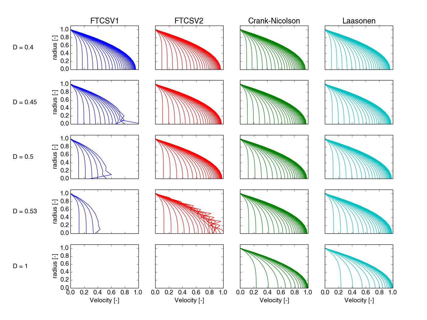
In Fig. 101 we see that the stability-limit for the two version is different for the to versions of treating the BC, for FTCS. Using L'Hopital's rule for r=0 give a smaller stability-limit, and we see that unstability arises at r=0, before the general stability-limit for the FTCS scheme (\( D=1/2 \)).
# Theta-scheme and using 2nd order forward difference for r=0
def thetaScheme_numpy_V2(theta, D, N, wOld):
    """ Algorithm for solving w^(n+1) for the startup of pipeflow
        using the theta-schemes. 2nd order forward difference is used
        on the von-Neumann bc at r=0.

        Args:
            theta(float): number between 0 and 1. 0->FTCS, 1/2->Crank, 1->Laasonen
            D(float): Numerical diffusion number [dt/(dr**2)]
            N(int): number of parts, or dr-spaces.
            wOld(array): The entire solution vector for the previous timestep, n.

        Returns:
            wNew(array): solution at timestep n+1
    """
    superDiag = np.zeros(N - 2)
    subDiag = np.zeros(N - 2)
    mainDiag = np.zeros(N-1)

    RHS = np.zeros(N - 1)

    j_array = np.linspace(0, N, N + 1)
    tmp = D*(1. - theta)

    superDiag[1:] = -D*theta*(1 + 0.5/j_array[2:-2])
    mainDiag[1:] = np.ones(N - 2)*(1 + 2*D*theta)
    subDiag[:] = -D*theta*(1 - 0.5/j_array[2:-1])

    a = tmp*(1 - 1./(2*j_array[2:-1]))*wOld[1:-2]
    b = (1 - 2*tmp)*wOld[2:-1]
    c = tmp*(1 + 1/(2*j_array[2:-1]))*wOld[3:]

    RHS[1:] = a + b + c

    superDiag[0] = -(4./3)*D*theta
    mainDiag[0] = 1 + (4./3)*D*theta
    RHS[0] = (1 - (4./3)*tmp)*wOld[1] + (4./3)*tmp*wOld[2]

    A = scipy.sparse.diags([subDiag, mainDiag, superDiag], [-1, 0, 1], format='csc')

    wNew = scipy.sparse.linalg.spsolve(A, RHS)
    w_0 = (1./3)*(4*wNew[0] - wNew[1])

    wNew = np.append(w_0, wNew)
    wNew = np.append(wNew, 0)


    return wNew
Figure 101: Results for stability tests performed for the two versions of the FTCS scheme, the Crank-Nicolson and the Laasonen schemes. Note that version 1 of FTCS scheme develops instabilities before \( D=0.5 \), and that instabilities start at \( r=0 \). For version 2 of FTCS scheme instability occurs for \( D=0 \).5 and for all values of \( r \), as expected.
Animation of numerical results obtained using three numerical schemes as well as the analytical solution.
emfs /src-ch5/ #python #package startup.py @ git@lrhgit/tkt4140/src/src-ch5/startup_compendium.py; Visualization.py @ git@lrhgit/tkt4140/src/src-ch5/Visualization.py; Startupfuncs.py @ git@lrhgit/tkt4140/src/src-ch5/Startupfuncs.py