Numerical Methods for Engineers

2.13 Variable time stepping methods

Recall the local truncation error of the Euler scheme applied to the model exponential decay equation (2.118), computed in (2.124) $$ \begin{align} \tau^{euler}_n = \frac{1}{2} h y''(x_n). \nonumber \end{align} $$

The error of the numerical approximation depends on $ h $ in a linear fashion, as expected for a first order scheme. However, the approximation error does also depend on the solution itself, more precisely on its second derivative. This is a property of the problem and we have no way of intervening on it. If one wants to set a maximum admissible error, then the only parameter left is the time step $ h $. The wisest manner to use this freedom is to adopt a variable time-stepping strategy, in which the time step is adapted according to estimates of the error as long as one advances in $ x $. Here we briefly present one possible approach, namely the 5-th order Runge-Kutta-Fehlberg scheme with variable time step (RKF45), as presented for example in [5]. Schematically, the main steps for implementing such scheme are listed bellow:

Assuming that the solution at $ x_n $ is available, compute a fourth and a fifth order RKF solution at time $ x_{n+1} $

Compute an estimate of the error: $ e_{n+1} \approx |y^{RKF5}_{n+1} - y^{RKF4}_{n+1}| $

Increase or decrease $ h $ according to pre-defined maximum and minimum admissible errors.

# src-ch1/fixed_vs_variable.py;

import numpy as np
import matplotlib.pyplot as plt


# Solve
# y' = beta * y
# y(0) = 1.
# with explicit Euler (fixed h) and RKF45

# ode coefficient
beta = -10.
# ode initial condition
y0 = 1.
# time step for Euler's scheme
h = 0.02
# domain
xL = 0.
xR = 1.
# number of intervals for Euler's scheme
N = int((xR-xL)/h)
# correct h for Euler's scheme
h = (xR-xL)/float(N)
# independent variable array for Euler's scheme
x = np.linspace(xL,xR,N)
# unknown variable array for Euler's scheme
y = np.zeros(N)
# x for exact solution
xexact = np.linspace(xL,xR,max(1000.,100*N))

# ode function
def f(x,y):
    return beta * y

# exact solution
def exact(x):
    return y0*np.exp(beta*x)

# Euler's method increment
def eulerIncrementFunction(x,yn,h,ode):
    return ode(x,yn)

# RKF45 increment
def rkf45step(x,yn,h,ode):
    # min and max time step
    hmin = 1e-5
    hmax = 5e-1
    # min and max errors
    emin = 1e-7
    emax = 1e-5
    # max number of iterations
    nMax = 100
    # match final time
    if x+h > xR:
        h = xR-x
    # loop to find correct error (h)
    update = 0
    for i in range(nMax):
        k1 = ode(x,yn)
        k2 = ode(x+h/4.,yn+h/4.*k1)
        k3 = ode(x+3./8.*h,yn+3./32.*h*k1+9./32.*h*k2)
        k4 = ode(x+12./13.*h,yn+1932./2197.*h*k1-7200./2197.*h*k2+7296./2197.*h*k3)
        k5 = ode(x+h,yn+439./216.*h*k1-8.*h*k2+3680./513.*h*k3-845./4104.*h*k4)
        k6 = ode(x+h/2.,yn-8./27.*h*k1+2.*h*k2-3544./2565.*h*k3+1859./4140.*h*k4-11./40.*h*k5)
        # 4th order solution
        y4 = yn + h * (25./216*k1 + 1408./2565.*k3+2197./4104.*k4-1./5.*k5)
        # fifth order solution
        y5 = yn + h * (16./135.*k1 + 6656./12825.*k3 + 28561./56430.*k4 - 9./50.*k5 +2./55.*k6)
        # error estimate
        er = np.abs(y5-y4)

        if er < emin:
            # if error small, enlarge h, but match final simulation time
            h = min(2.*h,hmax)            
            if x+h > xR:
                h = xR-x
                break
        elif er > emax:
            # if error big, reduce h
            h = max(h/2.,hmin)
        else:
            # error is ok, take this h and y5
            break

    if i==nMax-1:
        print("max number of iterations reached, check parameters")
        
    return x+h, y5, h , er
    
# time loop for euler
y[0] = y0
for i in range(N-1):
    y[i+1] = y[i] + h * eulerIncrementFunction(x[i],y[i],h,f)


# time loop for RKF45
nMax = 1000

xrk = np.zeros(1)
yrk = y0*np.ones(1)
hrk = np.zeros(1)
h = 0.5

for i in range(nMax):
    xloc , yloc, h , er = rkf45step(xrk[-1],yrk[-1],h,f)
    xrk = np.append(xrk,xloc)
    yrk = np.append(yrk,yloc)
    if i==0:
        hrk[i] = h
    else:
        hrk = np.append(hrk,h)
    if xrk[-1]==xR:
        break

plt.subplot(211)
plt.plot(xexact,exact(xexact),'b-',label='Exact')
plt.plot(x,y,'rx',label='Euler')
plt.plot(xrk,yrk,'o', markersize=7,markeredgewidth=1,markeredgecolor='g',markerfacecolor='None',label='RKF45')
plt.xlabel('x')
plt.ylabel('y(x)')
plt.legend()
plt.subplot(212)
plt.plot(xrk[1:],hrk,'o', markersize=7,markeredgewidth=1,markeredgecolor='g',markerfacecolor='None',label='RKF45')
plt.ylabel('h')
plt.legend(loc='best')
#plt.savefig('fixed_vs_variable.png')
plt.show()

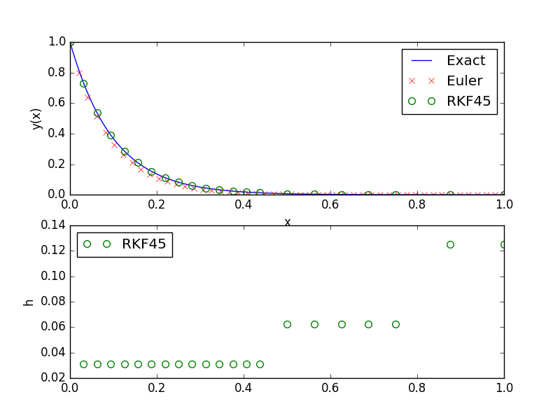
Figure 20: Numerical solution for the model exponential decay equation (2.118) using the Euler scheme and the RKF45 variable time step scheme (top panel) and time step used at each iteration by the variable time stepping scheme (bottom panel).