3.3.1 Example: Freezing of a water pipe
A dry layer of soil at initial temperature \( 20 ^{\circ} C \), is in a cold period exposed to a surface temperature of \( -15 ^{\circ} C \) in 30 days and nights. The question of concern is how deep the waterpipe must be located in order to avoid that the water in the pipe starts freezing?
The thermal diffusivity is \( \alpha = 5 \cdot 10^{-4} \) $m^2/hour$. With reference to (3.81) we have \( T_0=-15 ^{\circ} C \) and \( T_s=20 ^{\circ} C \), and \( \tau=30 \) days and nights \( =720 \) hours, and water freezes at \( 0 ^{\circ} C \).
From (3.83): $$ \begin{equation*} u=\frac{T-T_0}{T_s-T_0} =\frac{0-(-15)}{20-(-15)} =\frac{3}{7} =0.4286 \end{equation*} $$
Some values for \( \text{erf} (\eta) \) are tabulated below :
| \( x \) | \( \text{erf}(\eta) \) | \( \eta \) | \( \text{erf} (\eta) \) |
| 0.00 | 0.00000 | 1.00 | 0.84270 |
| 0.20 | 0.22270 | 1.20 | 0.91031 |
| 0.40 | 0.42839 | 1.40 | 0.95229 |
| 0.60 | 0.60386 | 1.60 | 0.97635 |
| 0.80 | 0.74210 | 1.80 | 0.98909 |
From the tabulated values for \( erf(x) \) and (3.101) we find \( \text{erf} (\eta)=0.4286\to \eta \approx 0.4 \) which according to (3.93) yields: $$ \begin{equation*} X=0.4\cdot2\sqrt{\tau\cdot\alpha}=0.8\cdot\sqrt{720\cdot5\cdot10^{-4}}=0.48 \text{m} \end{equation*} $$
While we have used a constant value for the diffusivity \( \alpha \), in can vary in the range \( \alpha \in [3 \, 10^{-4} \ldots 10^{-3}] \) \( m^2/s \), and the soil will normally contain some humidity.
3.3.2 Example: Stokes' first problem: flow over a suddenly started plate
Analytical solutions of the Navier-Stokes equations may be found only for situations for which some simplifying assumptions are made for the flow field, geometry etc. Several solutions are known for laminar flow due to moving boundaries and these are often used to illustrate the viscous boundary layer behaviour of such flow regimes.
In this example we illustrate Stokes' first problem flow over a suddenly started plate. Consider a quiescent fluid at time \( \tau < 0 \) resting on a plate parallel to the \( X \)-axis (see 44).
Figure 44: Stokes' first problem: flow over a suddenly started plate.

At time \( \tau=0 \) the plate is accelerated up to a constant velocity \( U=U_0 \), which allows for a parallel-flow assumption of \( V=0 \), \( W=0 \), for the velocity components orthogonal to \( U \). $$ \begin{equation} \frac{\partial U}{\partial\tau}+U \frac{\partial U}{\partial X}+V \frac{\partial U}{\partial Y}=-\frac{1}{\rho}\frac{\partial p}{\partial X}+ \nu\left(\frac{\partial^2 U}{\partial X^2}+\frac{\partial^2U}{\partial Y^2}\right) \tag{3.104} \end{equation} $$
A more detailed derivation is provided in appendix B in Numeriske Beregninger). Sufficiently far downstream one may further assume that the flow field is independent of the streamwise coordinate \( X \) too, i.e. \( U=U(Y,\tau) \), and the (3.104) reduces to: $$ \begin{equation} \frac{\partial U}{\partial\tau}=\nu \frac{\partial^2U}{\partial Y^2},\ 0 < Y < \infty \tag{3.105} \end{equation} $$
The assumption of a suddenly started plate implies the initial condition: $$ \begin{equation} U(U,0)=0 \tag{3.106} \end{equation} $$
and the assumptions of no slip at the plate and a quiescent fluid far away from the wall implies the following boundary conditions: $$ \begin{equation} \tag{3.107} \left.\begin{matrix} &U(0,\tau)=U_0 &U(\infty,\tau)=0 \end{matrix}\right.\ \end{equation} $$
To present the problem given by (3.105), (3.106), and (3.107) in an even more convenient manner we introduce the following dimensionless variables: $$ \begin{equation} u=\frac{U}{U_0},\ y=\frac{Y}{L},\ t=\frac{\tau\cdot\nu}{L^2} \tag{3.108} \end{equation} $$
where \( U_0 \), \( L \) are characteristic velocity and length, respectively. Further, substitution of (3.108) in (3.105) yields the following equation: $$ \begin{equation} \frac{\partial u}{\partial t}=\frac{\partial^2u}{\partial y^2},\ 0 < y < \infty \tag{3.109} \end{equation} $$
with corresponding initial condition: $$ \begin{equation} u(y,0)=0 \tag{3.110} \end{equation} $$
and boundary conditions $$ \begin{equation} \tag{3.111} \left.\begin{matrix} &u(0,t)=1 \\ &u(\infty,t)=0 \end{matrix}\right.\ \end{equation} $$
We now realize that the Stokes' first problems is the same as the on given by (3.84) and (3.85), save for a substitution of \( 0 \) and \( 1 \) in the boundary conditions. . The solution of (3.109) and (3.110) and the appropriate boundary conditions (3.111) is: $$ \begin{equation} u(y,t)=1-\text{erf}(\eta)=\text{erfc}(\eta)=\text{erfc}\left( \frac{y}{2\sqrt{t}}\right) \tag{3.112} \end{equation} $$
which has the following expression in physical variables: $$ \begin{equation} U(Y,\tau)=U_0\text{erfc} \left(\frac{Y}{2\sqrt{\tau\cdot\nu}}\right) \tag{3.113} \end{equation} $$
3.3.3 Example: The Blasius equation
The Blasius equation is a nonlinear ODE which may be derived as a simplification of the Navier-Stokes equations for the particular case of stationary, incompressible boundary layer flows.
Figure 45: Boundary layer development over a horizontal plate. {fig:216}

Detailed derivations of the Blasius equation may be found in numerous text in fluid mechanics concerned with boundary layer flow (appendix C, section C.2 in Numeriske Beregninger). However, for the sake of completeness we provide a brief derivation of the Blasius equation in the following. A stationary, incompressible boundary layer flow is governed by a simplified version of the Navier-Stokes equations (see equation (C.1.10), appendix C in Numeriske Beregninger).
For this particular flow regime, conservation of mass corresponds to: $$ \begin{equation} \frac{\partial u}{\partial x}+\frac{\partial v}{\partial y}=0 \tag{3.114} \end{equation} $$
whereas balance of linear momentum is ensured by: $$ \begin{equation} u \frac{\partial u}{\partial x}+v \frac{\partial u}{\partial y}=-\frac{1}{\rho}\frac{dp}{dx}+\nu\frac{\partial^2u}{\partial y^2} \tag{3.115} \end{equation} $$
For the case of a constant free stream velocity \( U=U_0 \) we may show that the streamwise pressure gradient \( \frac{dp}{dx}=0 \). (see equation (C.1.8) in appendix C in Numeriske Beregninger), and the equation {eq:23028}) reduces to: $$ \begin{equation} u \frac{\partial u}{\partial x}+v \frac{\partial u}{\partial y}=\nu\frac{\partial^2u}{\partial y^2} \tag{3.116} \end{equation} $$
with corresponding boundary conditions: $$ \begin{align} u(0)=0 \tag{3.117}\\ u\to U_0 \ & \text{for} \ y\to \delta \tag{3.118} \end{align} $$
In two dimensions, the mass conservation (3.114) may conveniently be satisfied by the introduction of a stream function \( \psi(x,y) \), defined as: $$ \begin{equation} u=\frac{\partial\psi}{\partial y},\ v=-\frac{\partial \psi}{\partial x} \tag{3.119} \end{equation} $$
The introduction of a similarity variable \( \eta \) and the non-dimensional stream function \( f \) $$ \begin{equation} \eta=\sqrt{ \frac{U_0}{2\nu x} }\cdot y \qquad \text{og} \qquad f(\eta)=\frac{\psi}{\sqrt{2U_o\nu x}} \tag{3.120} \end{equation} $$
we may transform the PDE in equation (3.120) to an ODE, which is the famous Blasius equation, for \( f \): $$ \begin{equation} f'''(\eta)+ f(\eta)\cdot f''(\eta)=0 \tag{3.121} \end{equation} $$
where we use the conventional notation \( \frac{df}{d\eta}\equiv f'(\eta) \) and similar for higher order derivatives.
The physical velocity components may be derived from the stream function by: $$ \begin{equation} \frac{u}{U_0}=f'(\eta),\ \frac{v}{U_0}=\frac{\eta \cdot f'(\eta)-f(\eta)}{\sqrt{2Re_x}} \tag{3.122} \end{equation} $$
where the Reynolds number has been introduced as $$ \begin{equation} Re_x=\frac{U_0x}{\nu} \tag{3.123} \end{equation} $$
The no slip condition \( u=0 \) for \( y=0 \) will consequently correspond to \( f'(0)=0 \) ad \( f'(\eta)=\frac{u}{U_0} \) in equation (3.122).
In absence of suction and blowing at the boundary for \( \eta= 0 \), the other no slip condition, i.e \( v=0 \) for \( \eta=0 \), corresponds to \( f(0)= 0 \) from equation (3.122). Further, the condition for the free stream of \( u\to U_0 \) from equation (3.118), corresponds to \( f'(\eta)\to 1 \) for \( \eta\to\infty \).
Consequently, the boundary conditions for the boundary layer reduce to: $$ \begin{equation} f(0)=f'(0)=0,\ f'(\eta_\infty)=1 \tag{3.124} \end{equation} $$
The shear stress at the wall may be computed from: $$ \begin{equation} \tau_{xy}=\mu U_0 \, f''(\eta)\sqrt{ \frac{U_0}{2\nu x}} \tag{3.125} \end{equation} $$
Numerical solution
The ODE in equation (3.121) with the boundary conditions in (3.124) represent a boundary value problem which we intend to solve with a shooting technique. We start by writing the third order, nonlinear ODE as a set of three, first order ODEs: $$ \begin{align} f_0'&=f_1 \nonumber \\ f_1'&=f_2 \tag{3.126}\\ f_2'&=-f_0 \, f_2 \nonumber \end{align} $$
where \( f_0=f \) and the corresponding boundary values are represented as $$ \begin{align} f_0(0)&=f_1(0)=0 \tag{3.127} \\ f_1(\eta_\infty)&=1 \nonumber \end{align} $$
As \( f''(0) \) is unknown we must find the correct value with the shooting method, \( f''(0)=f_2(0)=s \). Note that \( s \), which for the Blasius equation corresponds to the wall shear stress, must be chosen such that the boundary condition \( f_1(\eta_\infty)=1 \) is satisfied. We formulate this condition mathematically by introducing the boundary value error function \( \phi \): $$ \begin{equation} \phi(s)=f_1(\eta_\infty;s)-1 \tag{3.128} \end{equation} $$
As the system of ODEs in equation (3.126) is nonlinear, we follow in the procedure as outlined in 3.2 Shooting methods for boundary value problems with nonlinear ODEs, and use the secant method to find the correct initial value \( s= s^* \) such that the boundary value error function is zero \( \phi(s^*)=0 \).
Iteration procedure
The boundary value error function \( \phi \) in (3.128) is a nonlinear function of \( s \) (due to the nonlinear ODE it is derived from), and therefore, we must iterate to find the correct value.
Two initial guesses \( s^0 \) and \( s^1 \) are needed to start the iteration process, where the superscript is an iteration counter. Consequently, \( s^m \) refer to the \( s \)-value after the \( m \)-th iteration. In accordance with the generic procedure in (3.64) we find it more convenient to introduce the \( \Delta s \): $$ \begin{equation} s^{m+1}=s^m+\Delta s,\qquad \Delta s=-\phi(s^m)\cdot \left[\frac{s^m-s^{m-1}}{\phi(s^m)-\phi(s^{m-1})}\right],\ m=1,2.\dots \tag{3.129} \end{equation} $$
To formulate the iteration procedure we assume two values \( s^{m-1} \) \( s^m \) to be know, which initially correspond to \( s^0 \) and \( s^1 \). The iteration procedure the becomes:
- Compute \( \phi (s^{m-1}) \) and \( \phi (s^m) \) by solving (3.126).
- Compute \( \Delta s \) and \( s^{m+1} \) from (3.129)
- Update
- \( s^{m-1}\gets s^m \)
- \( s^m \gets s^{m+1} \)
- \( \phi (s^{m-1}) \gets \phi (s^m) \)
- Repeat 1-3 until convergence
Note that the convergence criteria is \( \Delta s < \varepsilon \), i.e. a test on the absolute value of \( \Delta s \), whereas a relative metric would be \( \left|\dfrac{\Delta s}{s}\right| \).
For some problems it may be difficult to guess appropriate initial guesses \( s^0 \) and \( s^1 \) to start the iteration procedure.
A very simple procedure to get an overview of the zeros for a generic function is to plot it graphically. In Figure 46 we have plotted \( \phi(s) \) for a very wide range \( s\in[0.05, 5.0] \).
Figure 46: Exploration of the error function \( \phi \) as a function of \( s \) for the Blasius equation.
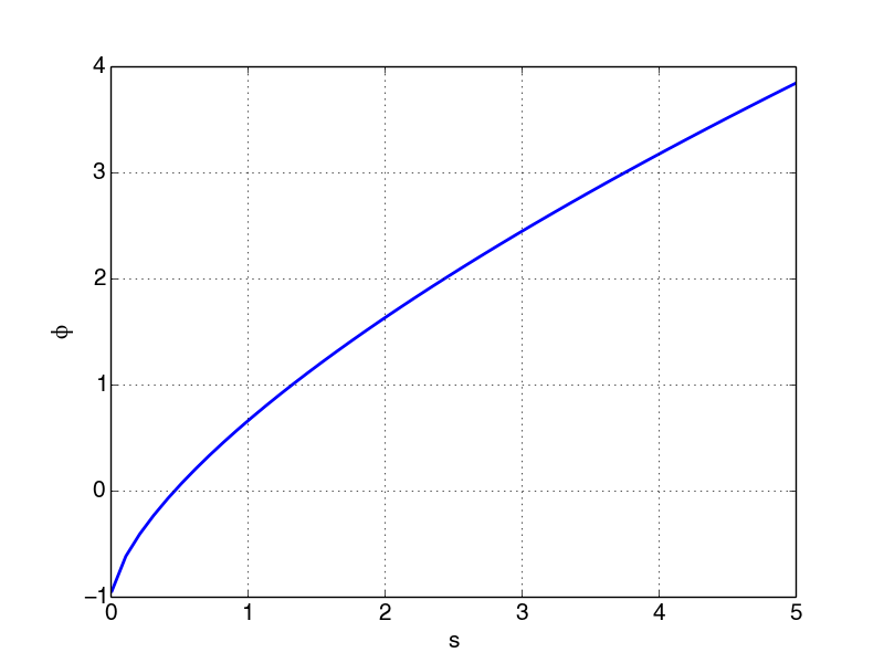
The computations of \( \phi \) were performed with the code
phi_plot_blasius_shoot_v2.py, and by visual inspection we observe
that the zero is in the range \( [0.45,0.5] \), i.e. much more narrow that
our initial guess.
# src-ch2/phi_plot_blasius_shoot_v2.py;ODEschemes.py @ git@lrhgit/tkt4140/src/src-ch2/ODEschemes.py;


from ODEschemes import euler, heun, rk4
from matplotlib.pyplot import *
# Change some default values to make plots more readable on the screen
LNWDT=3; FNT=20
matplotlib.rcParams['lines.linewidth'] = LNWDT; matplotlib.rcParams['font.size'] = FNT

def fblasius(y, x):
    """ODE-system for the Blasius-equation"""
    return [y[1],y[2], -y[0]*y[2]]

solvers = [euler, heun, rk4] #list of solvers
solver=solvers[2] # select specific solver


from numpy import linspace, exp, abs
xmin = 0
xmax = 5.75

N = 50  # no x-values
x = linspace(xmin, xmax, N+1)

# Guessed values
#s=[0.1,0.8]
s_guesses=np.linspace(0.01,5.0)

z0=np.zeros(3)

beta=1.0 #Boundary value for eta=infty

phi = []
for s_guess in s_guesses:
    z0[2] = s_guess
    u = solver(fblasius, z0, x)
    phi.append(u[-1,1] - beta)

plot(s_guesses,phi)

title('Phi-function for the Blasius equation')
ylabel('phi')
xlabel('s')
grid(b=True, which='both')
show()
Once appropriate values for \( s^0 \) and \( s^1 \) have been found we are
ready to find the solution of the Blasius equation with the shooting
method as outlined in blasius_shoot_v2.py.
# src-ch2/blasius_shoot_v2.py;ODEschemes.py @ git@lrhgit/tkt4140/src/src-ch2/ODEschemes.py;

from ODEschemes import euler, heun, rk4
from matplotlib.pyplot import *
# Change some default values to make plots more readable on the screen
LNWDT=3; FNT=20
matplotlib.rcParams['lines.linewidth'] = LNWDT; matplotlib.rcParams['font.size'] = FNT

def fblasius(y, x):
    """ODE-system for the Blasius-equation"""
    return [y[1],y[2], -y[0]*y[2]]


def dsfunction(phi0,phi1,s0,s1):
    if (abs(phi1-phi0)>0.0):
        return    -phi1 *(s1 - s0)/float(phi1 - phi0)
    else:
        return 0.0

solvers = [euler, heun, rk4] #list of solvers
solver=solvers[0] # select specific solver


from numpy import linspace, exp, abs
xmin = 0
xmax = 5.750

N = 400  # no x-values
x = linspace(xmin, xmax, N+1)

# Guessed values
s=[0.1,0.8]


z0=np.zeros(3)
z0[2] = s[0]


beta=1.0 #Boundary value for eta=infty

## Compute phi0

u = solver(fblasius, z0, x)
phi0 = u[-1,1] - beta

nmax=10
eps = 1.0e-3
for n in range(nmax):
    z0[2] = s[1]
    u = solver(fblasius, z0, x)
    phi1 = u[-1,1] - beta
    ds = dsfunction(phi0,phi1,s[0],s[1])
    s[0]  = s[1]
    s[1]  += ds
    phi0 = phi1
    print('n = {}  s1 = {} and ds = {}'.format(n,s[1],ds))

    if (abs(ds)<=eps):
        print('Solution converged for eps = {} and s1 ={} and ds = {}. \n'.format(eps,s[1],ds))
        break


plot(u[:,1],x,u[:,2],x)
xlabel('u og u\'')
ylabel('eta')


legends=[]
legends.append('velocity')
legends.append('wall shear stress')
legend(legends,loc='best',frameon=False)
title('Solution of the Blaisus eqn with '+str(solver.__name__)+'-shoot')
show()
close() #Close the window opened by show()
Figure 47: Solutions of the Blasius equation: dimensionless velocity \( f'(\eta) \) and shear stress \( f''(\eta) \).

In Figure 47 the dimensionless velocity \( f'(\eta) \) and shear stress \( f''(\eta) \) are plotted. The maximal \( f''(\eta) \) is occur for \( \eta=0 \) , which means that the maximal shear stress is at the wall.
Notice further that \( f'''(0)=0 \) means \( f''(\eta) \) has a vertical tangent at the wall.