5.2 First order partial differential equations

The left-hand side of the model equation, related to transport phenomena, consists of the term $ \dfrac{D()}{Dt} $, which is a 1st order partial differential equation (PDE). Let us look in detail at this term by considering the following equation: $$ \begin{equation} a \frac{\partial u}{\partial x}+b \frac{\partial u}{\partial y}+c=0 \tag{5.12} \end{equation} $$ If $ a $ or $ b $ are functions of $ x,\ y $ and $ u $, the equation is quasi-linear. When $ a $ and $ b $ are functions of $ x $ and/or $ y $, or constant, the function is linear.

The equation is non-linear if $ a $ or $ b $ are functions of either $ u $, $ \dfrac{\partial u}{\partial x} $ and/or $ \dfrac{\partial u}{\partial y} $. For example, the transport terms of the Navier-Stokes equations, i.e. the left-hand side of (5.3), are quasi-linear 1st order PDEs, even if we normally call them non-linear.

Writing (5.12) as: $$ \begin{equation} a\left(\frac{\partial u}{\partial x}+\frac{b}{a}\frac{\partial u}{\partial y}\right)+c=0 \tag{5.13} \end{equation} $$ Assuming that $ u $ is continuously differentiable: $$ \begin{equation*} du=\frac{\partial u}{\partial x}dx+\frac{\partial u}{\partial y}dy\to \frac{du}{dx}=\frac{\partial u}{\partial x}+ \frac{dy}{dx}\frac{\partial u}{\partial y} \end{equation*} $$ Defines the characteristic of (5.12) by: $$ \begin{equation} \frac{dy}{dx}=\frac{b}{a} \tag{5.14} \end{equation} $$

(5.14) inserted above provides: $$ \begin{equation*} a\left(\frac{\partial u}{\partial x}+\frac{b}{a}\frac{\partial u}{\partial y}\right)=a \frac{du}{dx} \end{equation*} $$ which further provides: $$ \begin{equation} a\cdot du+c\cdot dx=0 \tag{5.15} \end{equation} $$ Along the characteristic curve defined by $ \frac{dy}{dx}=\frac{b}{a} $, (5.12) reduces to an ODE given by (5.15). (5.15) is called the compatibility equation for (5.12). If (5.12) is linear, we can in principle first find the characteristic and then solve (5.15). This is normally not possible when (5.12) is quasi-linear or non-linear because in that case $ \frac{dy}{dx} $ is a function of $ u $, ie: of the solution itself.

5.2.1 Example 1:

The advection equation (5.7) given by $ \frac{\partial u}{\partial t}+a_0 \frac{\partial u}{\partial x} $ has the solution $ u(x,t)=f(x-a_0t) $, which is a wave propagating with constant profile and velocity along x. The wave moves to the right for $ a_0> 0 $. The characteristic is given here by: $ \frac{dx}{dt}=a_0 $.

This equation can be integrated directly, yielding: $ x=a_0t+C_1 $. Constant $ C_1 $ can be determined, for example, by noting that: $ x=x_0 $ for $ t=0 $, which implies that $ C_1=x_0 $. The characteristic curve equation becomes $ x=a_0t+x_0 $. (5.15) with $ c= 0 $ and $ a=1 $ results in $ du=0 $ . This means that $ u $ is here the particle velocity, which is constant along the characteristic.

Let us see an example with initial conditions, choose: $$ \begin{equation*} u(x,0)= \begin{cases} 1-x^2 \ \text{for} \ |x|\leq1 \\ 0 \text{for} \ |x| > 1 \end{cases} \end{equation*} $$

This is a parabola. From $ u(x,t)=f(x-a_0t) $ one has that $ u(x,0)=f(x) $. With $ \zeta=x-a_0t $, we can write the solution: $$ \begin{equation*} u(x,t)= \begin{cases} 1-\zeta^2 \ \text{for} \ |\zeta|\leq1 \\ 0 \ \text{for} \ |\zeta|>1 \end{cases} \end{equation*} $$ When we use $ \zeta $ as variable, the solution is stationary: we follow the wave. Figure 66 summarizes the example.

Figure 66: Propagation of initial condition by the linear advection equation.

5.2.2 Example 2:

The inviscid Burger's equation (5.8) is given by: $$ \begin{equation*} \frac{\partial u}{\partial t}+u\frac{\partial u}{\partial x}=0 \tag{5.16} \end{equation*} $$ This has the solution $ u(x,t)=f(x-u\cdot t) $ and characteristic curve given by: $ \frac{dx}{dt}=u $. This is the same solution as in the previous example, with the important difference that now $ a_0 $ is replaced with $ u $. The slope of characteristics varies now with $ x $, as indicated in Figure 67.

Figure 67: Characteristic curves for the Burger's equation (5.16) at different locations along $ x $.

The same initial condition as in the previous example provide the following solution: $$ \begin{equation*} u(x,t)= \begin{cases} 1-\zeta^2 \ \text{for} \ |\zeta|\leq1 \\ 0 \ \text{for} \ |\zeta|>1 \end{cases} \text{der}\ \zeta=x-u\cdot t \end{equation*} $$

Again, we see that the only difference from the previous example is that $ a_0 $ is now replaced by $ u $. Explicit solution, noting that $ u(x,t)=0 $ for $ |\zeta|>1 $: $$ \begin{align} u(x,t)=&\frac{1}{2t^2}[(2xt-1)\pm g(x,t)],\ \nonumber\\ g(x,t) =&\sqrt{1-4xt+4t^2},\ |\zeta|\leq1 \tag{5.17} \\ \frac{\partial u}{\partial x}=\frac{g(x,t)\pm1}{t\cdot g(x,t)} \tag{5.18} \end{align} $$

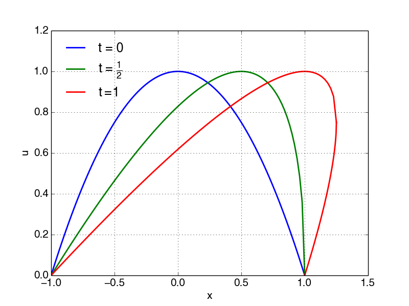
By this method of solution uniqueness is lost when characteristic intersect (Figure 68). In this case one has that $ u(x,t) $ takes two possible values for $ x\geq1 $, when $ \frac{\partial u}{\partial x}(1,t) > 0 $. The critical value $ t_{crit} $ when this occur takes place when $ \frac{\partial u}{\partial x}(1,t)\to\infty $, as one can conclude from (5.18), which implies that $ g(1,t)=0=1-2t\to t_{crit}=\frac{1}{2} $.

For $ t\leq \frac{1}{2} $ one uses (5.17) and (5.18) with positive sign for $ g(x,t) $ for all values of $ x $. For $ t>\frac{1}{2} $ the critical value arises at $ x^*=\frac{1+4t^2}{4t} $ with $ u^*=1-\frac{1}{4t^2} $. For $ -1\leq x\leq x^* $ one can still use (5.17) and (5.18) with positive sign for $ g(x,t) $, but for $ 1\leq x\leq x^* $ the lower part of the solution is given by using (5.17) and (5.18) with negative sign in front of $ g(x,t) $. The maximum value $ u_{maks}=1 $ is always given at $ x=t $.

In order to obtain a unique solution, one must introduce the concept of a moving discontinuity: in gas dynamics this is called a shock, in hydraulics a hydraulic jump.

Figure 68: Illustration of intersecting characteristic curves.

The characteristic curves shown in Figure 69 are given by: $$ \begin{equation*} x=(1-x_0^2)\cdot t+x_0,\ \text{der} \ x=x_0 \ \text{for} \ t=0 \end{equation*} $$

Figure 69: Inviscid Burger's equation solution. Note that solution for time $ t=1 $ is multiply. After $ t_{crit} $ additional mathematical notions have to be applied to identify a unique solution.