Exercise 8: Heat conduction in a triangle of two different materials
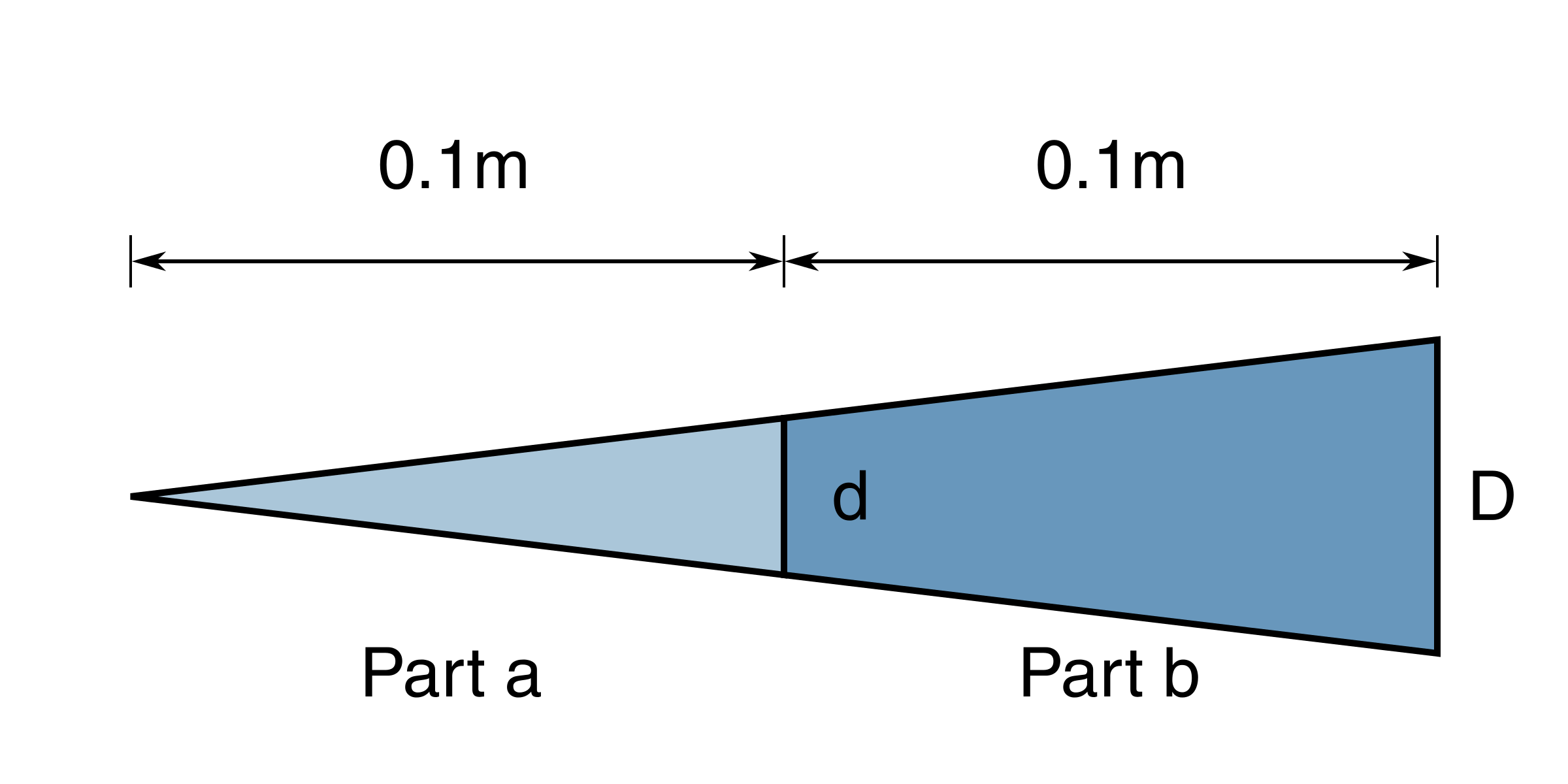
In this exercise we will look at a slightly more involved version of the trapezoidal cooling rib in 4.4.2 Cooling rib with variable cross-section which is illustrated in Figure 63. This cooling rib is composed av a triangle (part a) and a trapezoidal part (part b) which are made of materials of different heat properties. The purpose of this exercise is to illustrated how discontinuties in heat properties may be treated. We will find that that the temperature varies continuously along the rib, whereas the temperature gradient will have a discontinuity at the junction of the two materials.
Figure 63: A triangle of two different materials.
In appendix B of Numeriske metoder the quasi one-dimensional differential equation for heat conduction is derived: $$ \begin{equation*} -dQ_x = P \;h \;[T(X)-T_{\infty}]\;dX \qquad \text{ where } \quad Q_x = -kA\frac{dT}{dX} \end{equation*} $$
As \( dX \to 0 \) so will \( dQ \to 0 \) and consequently \( \Rightarrow Q = constant \) which means that at the cross-section between the two different materials we must satisfy the following relation: $$ \begin{equation} \tag{4.146} Q_a = Q_b \Rightarrow k_aA_a\left(\frac{dT}{dX}\right)_a = k_bA_b\left(\frac{dT}{dX}\right)_b \end{equation} $$
The the junction the cross-sectional areas of the two materials are the same \( A_a = A_b \) and there fore \( \left( \dfrac{dT}{dX} \right) _b = \dfrac{k_a}{k_b} \left( \dfrac{dT}{dX} \right)_a \), which may be rendered on dimensionless form by using (4.78): $$ \begin{equation} \left( \frac{d\theta}{dx}\right)_b = \frac{k_a}{k_b}\left( \frac{d\theta}{dX}\right)_a \tag{4.147} \end{equation} $$
Assume the following cooling rib geometry $$ \begin{equation} \begin{array}{l} L = 0.2m, \qquad D =0.02m, \qquad d=0.01m \tag{4.148} \end{array} \end{equation} $$
and let the thermodynamical properties be given by:
With these geometrical and thermodynamical properties equation junction condition in equation (4.147) is transformed to: $$ \begin{equation} \left( \dfrac{d\theta}{dx}\right)_b = 4\;\left( \dfrac{d\theta}{dx}\right) _a \tag{4.149} \end{equation} $$
whereas the differential equation for quasi onedimensional heat conduction remains: $$ \begin{equation} \frac{d}{dx}\left( \frac{x}{\beta^2}\frac{d\theta}{dx}\right) - \theta(x) = 0 \tag{4.150} \end{equation} $$
the expressions for \( \beta \) are: $$ \begin{equation} \beta^2 = \frac{2\bar{h}\;L^2}{D \;k} \tag{4.151} \end{equation} $$
which in our example corresponds to $$ \begin{equation} \beta^2_a = 2.0 \qquad \text{ and } \qquad \beta^2_b = 8.0 \tag{4.152} \end{equation} $$
By rendering equation (4.150) in this way we satisfy the continuity condition in equation (4.146).
The exercise is to solve the heat equation (4.150) numerically for the triangle in Figure 63 with the geometry and thermodynamical parameters given above.
Figure 64: Spatial discretization for the example of heat conduction in a triangle composed by two different materials with material interface at point \( M \).

Referring to Figure 64, we use the following numbering: $$ \begin{align} \tag{4.153} \begin{array}{l} x_i = (i-1)\;h \ , \ i=1,2,...,N+1 \textrm{ with } h = \frac{1}{N}\\ M = \frac{N}{2}+1 \textrm{ with N being an even number and }x_M = 0.5 \end{array} \end{align}$$
With \( k = k_a \) for \( i = M \) we get that \( \beta = \beta_a \) for \( i=1,2,...,M \) and \( \beta = \beta_b \) for \( i > M \). For \( i\not= M \) we can write (4.150) $$ \begin{equation} \tag{4.154} \frac{d}{dx}\left( x\frac{d\theta}{dx}\right) - \beta^2 \;\theta(x) = 0 \end{equation} $$
Discretizing (4.154) using (2.45) in Chapter (2 Initial value problems for Ordinary Differential Equations): $$ \begin{equation*} -x_{i- \frac{1}{2}} \;\theta_{i-1} + (x_{i+ \frac{1}{2}} + x_{i- \frac{1}{2}} + \beta^2 h^2) \;\theta_i - x_{i + \frac{1}{2}} \;\theta_{i+1} = 0 \end{equation*} $$
Noting that \( x_{i- \frac{1}{2}} = (i - \frac{3}{2}) \;h \) and \( x_{i+ \frac{1}{2}} = (i - \frac{1}{2})\;h \) we can write: $$ \begin{equation*} \left(i - \frac{3}{2}\right) \;\theta_{i-1} + [2(i-1) + \beta^2h] \;\theta_i - \left(i- \frac{1}{2} \right) \;\theta_{i+1} = 0 \end{equation*} $$
or divided by \( i \): $$ \begin{equation} \tag{4.155} \ - \left( 1-\frac{3}{2i} \right) \;\theta_{i-1} + \left[ 2 \;\left( 1 - \frac{1}{i} \right) + \frac{\beta^2h}{i} \right] \;\theta_i - \left(1 - \frac{1}{2i} \right) \;\theta_{i+1} = 0 \end{equation} $$
(4.155) is used for \( i = 2,3,...,N \), however, except for \( i = M = N/2+1 \).
For i \( = \) 1
From (4.82) we get the boundary condition for \( x=0 \): $$ \begin{equation} \dfrac{d\theta}{dx}(0)= \beta_a^2 \;\theta(0) \to \dfrac{-3 \theta_1 + 4 \theta_2 - \theta_3}{2h}= \beta_a^2 \;\theta_1, \tag{4.156} \end{equation} $$
where we have used forward differences (See forward).
This results in: $$ \begin{equation} \tag{4.157} \theta_3 = 4\theta_2 - (3 + 2h\beta_a^2) \;\theta_1 \end{equation} $$
Writing (4.155) for \( i= 2 \): $$ \begin{equation*} -\left(1- \frac{3}{4}\right) \;\theta_1 + \left[ 2\;\left(1 - \frac{1}{2}\right) + \frac{\beta_a^2h}{2}\right] \;\theta_2 - \left(1 - \frac{1}{4}\right) \;\theta_3 \end{equation*} $$
and considering (4.151) and (4.157) results in: $$ \begin{equation} \tag{4.158} \left( 1 + \frac{3h}{2}\right) \;\theta_1 - \left( 1 - \frac{h}{2}\right) \;\theta_2 = 0 \end{equation} $$
This is the first equation of our system.
For i \( = \) M.
Figure 65: Spatial discretization for the example of heat conduction in a triangle composed by two different materials with material interface at point \( M \). Detail of the discretization for the use of centered finite differences for point \( M \),

According to the discretization illustrated in Figure 65, here we use an equation of the form given in (4.150), which discretized using (2.45) from Chapter (2 Initial value problems for Ordinary Differential Equations), results in: $$ \begin{align*} \begin{array}{c} \beta_{M- \frac{1}{2}}^2 = \beta_a^2 = 2.0 \ , \ \beta_{M+\frac{1}{2}}^2 = \beta_b^2 = 8.0\\ x_{M-\frac{1}{2}} = \dfrac{h}{2}(N-1)= \dfrac{(1-h)}{2} \ , \ x_{M+\frac{1}{2}} = \dfrac{h}{2}(N+1) = \dfrac{(1+h)}{2} \end{array} \end{align*} $$
which provides: $$ \begin{equation} \tag{4.159} -4 \;(1-h) \;\theta _{M-1} + [5-3h+16h^2]\;\theta_M - (1+h) \;\theta_{M+1} = 0 \end{equation} $$
For i \( = \) N we can use (4.155) with \( \beta^2 = \beta_b^2 = 8.0 \): $$ \begin{equation} \tag{4.160} -\left(1-\frac{3h}{2}\right) \;\theta_{N-1} + 2 \;[(1-h)+4h^2] \;\theta_N = \left(1-\frac{h}{2}\right) \end{equation} $$
Equations (4.158)–(4.160) constitute a linear system of equations with a tridiagonal matrix and can be solved as such using the Thomas algorithm. In addition to the temperature, we also want to calculate the temperature gradient \( \theta'(x) \) . For \( x=0 \) we use (4.82) and interface condition \( \frac{d\theta}{dx}(0.5+)\equiv \left( \frac{d\theta}{dx}\right)_b \) found from (4.149). The other values are computed using standard central differences, besides for x \( = \) 0.5 og x \( = \) 1.0, where second order backward differences are used. Let us look at the use of the differential equation as an alternative.
We integrate (4.154): $$ \begin{equation} \tag{4.161} \frac{d\theta_i}{dx}=\frac{\beta^2}{x_i} \int_{x_1}^{x_i} \theta(x)dx \ , \ i= 2,3,...,N+1 \end{equation} $$
Integral \( I = \int_{x_1}^{x_i}\theta(x)dx \) can be calculated using the trapezium method, for example . The computation of (4.161) is shown below in pseudo-code form: $$ \begin{align*} \begin{array}{rrrlll} &&\theta_1' &:=& \beta_a^2\;\theta_1\\ &&s&:=& 0\\ &&\text{Utfør for } i&:=&2,...,N+1\\ &&x&:=&h \; (i-1)\\ &&s&:=&s+0.5h \; (\theta_i+\theta_{i-1})\\ \end{array} \end{align*} $$ $$ \begin{equation*} \text{Dersom $(i\le M)$ sett }\theta_i ':= \frac{\beta_a^2\;s}{x} \text{ ellers }\theta_i':= \frac{\beta_b^2 \;s}{x} \end{equation*} $$
In the following table we have used (4.161) and the trapezium method. In this case, the accuracy of the two methods for calculating \( \theta'(x) \) is quite similar as both \( \theta \) and \( \theta' \) are smooth functions (except at x \( = \) 0.5), but generally the integration method will be more accurate if there are discontinuities..
Solution of equation (4.150) with \( h = 0.01 \)
| x | \( \theta(x) \) | rel. feil | \( \theta'(x) \) | rel. feil |
| 0.00 | 0.08007 | 1.371E-4 | 0.16014 | 1.312E-4 |
| 0.10 | 0.09690 | 1.341E-4 | 0.17670 | 1.302E-4 |
| 0.20 | 0.11545 | 1.386E-4 | 0.19438 | 1.286E-4 |
| 0.30 | 0.13582 | 1.252E-4 | 0.21324 | 1.360E-4 |
| 0.40 | 0.15814 | 1.265E-4 | 0.23333 | 1.329E-4 |
| 0.45 | 0.17007 | 1.294E-4 | 0.24387 | 1.312E-4 |
| 0.5- | 0.18253 | 1.260E-4 | 0.25472 | 1.021E-4 |
| 0.5+ | 0.18253 | 1.260E-4 | 1.01889 | 1.021E-4 |
| 0.55 | 0.23482 | 5.962E-5 | 1.07785 | 1.067E-4 |
| 0.60 | 0.29073 | 5.848E-5 | 1.16297 | 9.202E-5 |
| 0.70 | 0.41815 | 3.348E-5 | 1.39964 | 7.288E-5 |
| 0.80 | 0.57334 | 1.744E-5 | 1.71778 | 5.938E-5 |
| 0.90 | 0.76442 | 7.849E-6 | 2.11851 | 4.862E-5 |
| 1.00 | 1.00000 | 0.0 | 2.60867 | 1.526E-4 |