8.9 Flux limiters

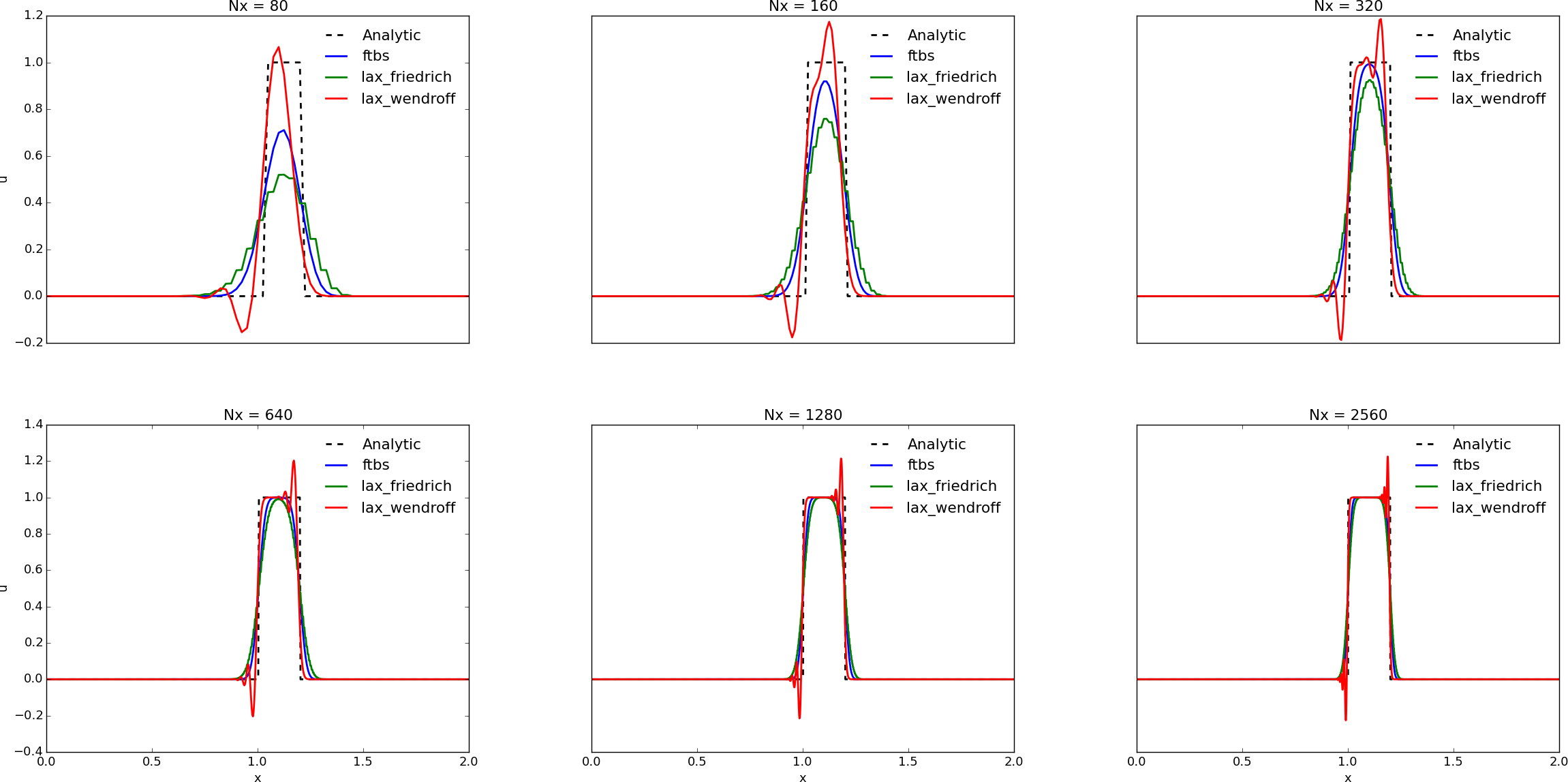
Looking at the previous examples and especially Figure 115 we clearly see the difference between first and second order schemes. Using a first order scheme require a very high resolution (and/or a cfl number close to one) in order to get a satisfying solution. What characterizes the first order schemes is that they are highly diffusive (loss of amplitude). Unless the resolution is very high or the cfl-number is very close to one, the first order solutions will lose amplitude as time passes. This is evident in the animation (video:sine). (To see how the different schemes behave with different combinations of CFL-number, and frequencies try the sliders app located in the git repository in chapter 6.) However if the solution contain big gradients or discontinuities, the second order schemes fail, and introduce nonphysical oscillations due to their dispersive nature. In other words the second order schemes give a much higher accuracy on smooth solutions, than the first order schemes, whereas the first order schemes behave better in regions containing sharp gradients or discontinuities. First order upwind methods are said to behave monotonically varying in regions where the solution should be monotone (cite:Second Order Positive Schemes by means of Flux Limiters for the Advection Equation.pdf). Figure 116 show the behavior of the different advection schemes in a solution containing discontinuities; oscillations arises near discontinuities for the Lax-Wendroff scheme, independent of the resolution. The dissipative nature of the first order schemes are evident in solutions with "low" resolution.

Figure 116: Effect of refining grid on a solution containing discontinuities; a square box moving with wave speed a=1. Solutions are showed at t=1, using a cfl-number of 0.8.

The idea of Flux limiters is to combine the best features of high and low order schemes. In general a flux limiter method can be obtained by combining any low order flux $ F_{l} $, and high order flux $ F_h $. Further it is convenient/required to write the schemes in the so the so-called conservative form as in (8.41) repeated here for convenience $$ \begin{align} u_j^{n+1} = u_j^{n} + \frac{\Delta t}{\Delta x} \left ( F_{j-1/2} - F_{j+1/2} \right ) \tag{8.60} \end{align} $$

The general flux limiter method solves (8.60) with the following definitions of the fluxes $ F_{i-1/2} $ and $ F_{i+1/2} $ $$ \begin{align} F_{j-1/2} = F_l(j-1/2) + \phi(r_{j-1/2})\big[F_h(j-1/2) - F_l(j-1/2)\big] \tag{8.61}\\ F_{j+1/2} = F_l(j+1/2) + \phi(r_{j+1/2})\big[F_h(j+1/2) - F_l(j+1/2)\big] \tag{8.62} \end{align} $$

where $ \phi(r) $ is the limiter function, and $ r $ is a measure of the smoothness of the solution. The limiter function $ \phi $ is designed to be equal to one in regions where the solution is smooth, in which $ F $ reduces to $ F_h $, and a pure high order scheme. In regions where the solution is not smooth (i.e. in regions containing sharp gradients and discontinuities ) $ \phi $ is designed to be equal to zero, in which $ F $ reduces to $ F_l $, and a pure low order scheme. As a measure of the smoothness, $ r $ is commonly taken to be the ratio of consecutive gradients $$ \begin{equation} r_{j-1/2} = \frac{u_{j-1}-u_{j-2}}{u_{j}-u_{j-1}}, \qquad r_{j+1/2} = \frac{u_{j}-u_{j-1}}{u_{j+1}-u_{j}} \tag{8.63} \end{equation} $$

In regions where the solution is constant (zero gradients), some special treatment of $ r $ is needed to avoid division by zero. However the choice of this treatment is not important since in regions where the solution is not changing, using a high or low order method is irrelevant.

8.9.0.1 Lax-Wendroff limiters

The Lax-Wendroff scheme for the advection equation may be written in the form of (8.60) by defining the Lax-Wendroff Flux $ F_{LW} $ as: $$ \begin{align} F_{LW}\left(j-1/2\right) = F_{LW}\left(u_{j-1}, u_{j}\right) = a\:u_{j-1} + \frac{1}{2}a\left(1-\frac{\Delta t}{\Delta x}a\right)\big[ u_{j}-u_{j-1}\big] \tag{8.64}\\ F_{LW}\left(j+1/2\right) = F_{LW}\left(u_{j}, u_{j+1}\right) = a\:u_{j} + \frac{1}{2}a\left(1-\frac{\Delta t}{\Delta x}a\right)\big[ u_{j+1}-u_{j}\big] \tag{8.65} \end{align} $$

which may be showed to be the Lax-Wendroff two step method condensed to a one step method as outlined in (8.7.1 Lax-Wendroff for non-linear systems of hyperbolic PDEs). Notice the term $ \frac{\Delta t}{\Delta x}a = c $. Now the Lax-Wendroff flux assumes that of an upwind flux ($ a\:u_{j-1} $ or $ a\:u_{j} $) with an additional anti diffusive term ($ \frac{1}{2}a\left(1-c\right)\big[ u_{j}-u_{j-1}\big] $ for $ F_{LW}\left(j-1/2\right) $). A flux limited version of the Lax-Wendroff scheme could thus be obtained by adding a limiter function $ \phi $ to the second term $$ \begin{align} F\left(j-1/2\right) = a\:u_{j-1} + \phi\left(r_{j-1/2}\right)\frac{1}{2}a\left(1-c\right)\big[ u_{j}-u_{j-1}\big] \tag{8.66}\\ F\left(j+1/2\right) = a\:u_{j} + \phi\left(r_{j+1/2}\right)\frac{1}{2}a\left(1-c\right)\big[ u_{j+1}-u_{j}\big] \tag{8.67} \end{align} $$

When $ \phi=0 $ the scheme is the upwind scheme, and when $ \phi=1 $ the scheme is the Lax-Wendroff scheme. Many different limiter functions have been proposed, the optimal function however is dependent on the solution.Sweby () showed that in order for the Flux limiting scheme to possess the wanted properties of a low order scheme; TVD, or monotonically varying in regions where the solution should be monotone, the following equality must hold $$ \begin{equation} 0 \leq \Big(\frac{\phi(r)}{r}, \phi(r)\Big) \leq 2 \tag{8.68} \end{equation} $$

Where we require $$ \begin{equation} \phi(r) = 0, \quad r\leq 0 \tag{8.69} \end{equation} $$

Hence for the scheme to be TVD the limiter must lie in the shaded region of Figure 117, where the limiter function for the two second order schemes, Lax-Wendroff and Warming and Beam are also plotted.

Figure 117: TVD region for flux limiters (shaded), and the limiters for the second order schemes; Lax-Wendroff, and Warming and Beam

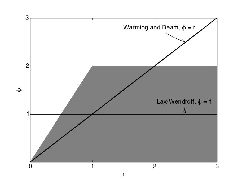
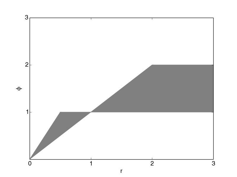
For the scheme to be second order accurate whenever possible, the limiter must be an arithmetic average of the limiter of Lax-Wendroff ($ \phi=1 $) and that of Warming and Beam($ \phi=r $) . With this extra constraint a second order TVD limiter must lie in the shaded region of Figure 118

Figure 118: Second order TVD region for flux limiters; Sweby diagram

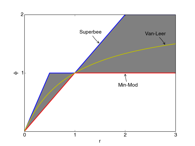
Note that $ \phi(0)=0 $, meaning that second order accuracy must be lost at extrema. All schemes pass through the point $ \phi(1)=1 $, which is a general requirement for second order schemes. Many limiters that pass the above constraints have been proposed. Here we will only consider a few: $$ \begin{align} Superbee: \quad \phi(r)=max\left(0,min(1,2r),min(2,r)\right) \tag{8.70}\\ Van-Leer: \quad \phi(r)=\frac{r+\lvert r \rvert}{1+\lvert r \rvert} \tag{8.71}\\ minmod: \quad \phi(r)=minmod(1,r) \tag{8.72} \end{align} $$

where minmod of two arguments is defined as $$ \begin{equation} minmod(a,b)= \left\{ \begin{array}{ll} a \quad if \quad a\cdot b > 0 \quad and \quad \lvert a \rvert > \lvert b \rvert \\ b \quad if \quad a\cdot b > 0 \quad and \quad \lvert b \rvert > \lvert a \rvert > 0 \\ 0 \quad if \quad a\cdot b < 0 \end{array} \right. \tag{8.73} \end{equation} $$ The limiters given in (8.70) -(8.72) are showed in Figure 119. Superbee traverses the upper bound of the second order TVD region, whereas minmod traverses the lower bound of the region. Keeping in mind that in our scheme, $ \phi $ regulates the anti diffusive flux, superbee is thus the least diffusive scheme of these.

Figure 119: Second order TVD limiters

In addition we will consider the two base cases: $$ \begin{align} upwind: \quad \phi(r)=0 \tag{8.74}\\ Lax-Wendroff: \quad \phi(r)=1 \tag{8.75} \end{align} $$ in which upwind, is TVD, but first order, and Lax-Wendroff is second order, but not TVD.

8.9.0.2 Example of Flux limiter schemes on a solution with continuos and discontinuous sections

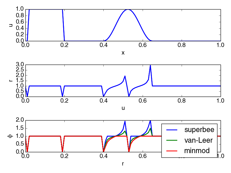
All of the above schemes have been implemented in the python class Fluxlimiters, and a code example of their application on a solution containing combination of box, and sine moving with wavespeed a=1, may be found in the python script advection-schemes-flux-limiters.py. The result may be seen in the video (video:Flux_limiters)

The effect of Flux limiting schemes on solutions containing continuos and discontinuous sections

Figure 120: Relationship between $ u $ and smoothness measure $ r $, and different limiters $ \phi $, on continuos and discontinuous solutions