8.5 Errors due to diffusion and dispersion

We have previously seen that the numerical amplification factor $ G $ is complex, i.e. it has a real part $ G_r $ and a imaginary part $ G_i $. Being a complex number $ G $ may be represented in the two traditional ways: $$ \begin{equation} G = G_r+i\cdot G_i = |G|\cdot e^{-i\phi} \tag{8.23} \end{equation} $$

where the latter is normally referred to as the polar form which provides a means to express $ G $ by the amplitude (or absolute value) $ |G| $ and the phase $ \phi $. $$ \begin{equation} |G|=\sqrt{G^2_r+G^2_i}, \qquad \phi = \arctan\left(\frac{-G_i}{G_r}\right) \tag{8.24} \end{equation} $$

I the section 7.4 Stability analysis with von Neumann's method we introduced the diffusion/dissipation error $ \varepsilon_D $ (dissipasjonsfeilen) as: $$ \begin{equation} \varepsilon_D = \frac{|G|}{|G_a|} \tag{8.25} \end{equation} $$

where $ |G_a| $ is the amplituden of analytical amplification factor $ G_a $, i.e. we have no dissipative error when $ \varepsilon_D = 1 $ .

For problems and models related with convection we also need to consider the error related with timing or phase, and introduce a measure for this kind error as the dispersion error $ \varepsilon_\phi $: $$ \begin{equation} \varepsilon_\phi = \frac{\phi}{\phi_a} \tag{8.26} \end{equation} $$

where $ \phi_a $ is the phase for the analytical amplification factor. And again $ \varepsilon_\phi = 1 $ corresponds to no dispersion error. Note for parabolic problems with $ \phi_a = 0 $ , it is common to use $ \varepsilon_\phi = \phi $.

8.5.1 Example: Advection equation

Consider the linear advection equation, given by: $$ \begin{equation*} \frac{\partial u}{\partial t} +a_0 \frac{\partial u}{\partial x}= 0 \end{equation*} $$

Similarly to what introduced in the section 7.4 Stability analysis with von Neumann's method, we use $$ \begin{equation} u(x,t) = e^{i(\beta x - \omega t)}, \tag{8.27} \end{equation} $$ with $ \omega = a_0\beta $, where $ \beta $ is the wave number. With the notation introduced above we get: $$ \begin{equation} u(x,t) = e^{i(\beta x -\omega t)} = e^{-i\cdot \phi_a} \ , \ \phi_a = \omega t - \beta x \tag{8.28} \end{equation} $$

From equation (7.39) in the section 7.4 Stability analysis with von Neumann's method: $$ \begin{equation*} G_a = \frac{u(x_j,t_{n+1})}{u(x_j,t_n)} = \frac{e^{i(\beta x_j -\omega t_{n+1})}}{e^{i(\beta x_j - \omega t_n)}} = \exp[i(\beta x_j - \omega t_{n+1})-i(\beta x_j - \omega t_n)] = \exp(-i\omega\cdot\Delta t) \end{equation*} $$

where we have inserted (8.28). Thus, $ |G_a|=1 \to \varepsilon_D = |G| $ .

Hence: $$ \begin{equation} \phi_a = \omega \cdot \Delta t = a_0 \beta \cdot \Delta t = a_0 \frac{\Delta t}{\Delta x}\beta \cdot \Delta x = C\cdot\delta \tag{8.29} \end{equation} $$

$ C $ is the Courant-number and $ \delta = \beta\cdot\Delta x $ as usual.

From (8.29) we also get: $$ \begin{equation} a_0 = \frac{\phi_a}{\beta \cdot \Delta t} \tag{8.30} \end{equation} $$

Analogously to (8.30), we can define a numerical propagation velocity $ a_{num} $: $$ \begin{equation} a_{num} = \frac{\phi}{\beta\cdot\Delta t} \tag{8.31} \end{equation} $$

The dispersion error in (8.26) can then be written as: $$ \begin{equation} \varepsilon_\phi = \frac{a_{num}}{a_0} \tag{8.32} \end{equation} $$

When the dispersion error is greater than one we have that the numerical propagation speed is greater than the physical one. This results in the fact that the numerical solution will move faster than the physical one. On the other hand, a $ \varepsilon_\phi < 1 $ results in slower numerical propagation speed compared to the physical one, with obvious consequences for the numerical solution.

Let us know have a closer look to the upwind scheme and the Lax-Wendroff scheme.

8.5.2 Example: Diffusion and dispersion errors for the upwind schemes

From equation (8.13) in the section 8.3 Upwind schemes: $$ \begin{equation} G=1+C\cdot(\cos(\delta)-1)-i\cdot C\sin(\delta)=G_r + i\cdot G_i \tag{8.33} \end{equation} $$

which inserted in (8.24) and (8.26) gives: $$ \begin{equation} \begin{array}{rcl} \varepsilon_D = |G| &= \sqrt{[1+C\cdot(\cos(\delta)-1)]^2+[C\sin(\delta)]^2}\\\\ &= \sqrt{1-4C(1-C)\sin^2(\frac{\delta}{2})} \end{array} \tag{8.34} \end{equation} $$ $$ \begin{equation} \varepsilon_\phi = \frac{\phi}{\phi_a}=\frac{1}{C\delta}\arctan\left[ \frac{C\sin(\delta)}{1-C(1-\cos(\delta))} \right] \tag{8.35} \end{equation} $$

Figure 108 shows (8.34) and (8.35) as a function of $ \delta $ for different Courant-number values. We see that $ \varepsilon_D $ decreases strongly for larger frequencies, which means that the numerical amplitude becomes much smaller than the exact one when use a large time step. This applies even for $ C = 0.8 $ . Remember that the amplitude factor for the $ n $-th time iteration is $ |G|^n $ (see also Figure 107). The scheme is performance is rather modest for general use even though it is stable.

For $ C=0.5 $ we have no dispersion errors. For $ C < 0.5 $ we have that $ \varepsilon_\phi < 1 $, so that the numerical propagation speed is smaller than the physical one $ a_0 $. On the other hand, for $ C > 0.5 $ we have that $ \varepsilon_\phi>1 $.

Figure 108: Diffusion error $ \varepsilon_D $ (left y-axis) and dispersion error $ \varepsilon_\phi $ (right y-axis) for the upwind scheme as a function of frequency for the upwind scheme. The dotted lines of $ \varepsilon_\phi $ correspond to same CFL-numbers as solid lines of $ \varepsilon_D $ with the same color.

8.5.3 Example: Diffusion and disperision errors for the Lax-Wendroff scheme

From equation (8.46): $$ \begin{equation} G = 1+C^2\cdot(\cos(\delta)-1)-i\cdot C\sin(\delta)=G_r+i\cdot G_i \tag{8.36} \end{equation} $$

which inserted in (8.24) and (8.26) gives: $$ \begin{equation} \begin{array}{rcl} \varepsilon_D = |G| &= \sqrt{ [1 + C^2 \cdot (\cos(\delta)-1)]^2 +(C\sin(\delta))^2 }\\\\ &= \sqrt{ 1 - 4C^2(1-C^2)\sin^4\left(\frac{\delta}{2}\right) } \end{array} \tag{8.37} \end{equation} $$ $$ \begin{equation} \varepsilon_\phi = \frac{\phi}{\phi_a} = \frac{1}{C\delta}\arctan\left[ \frac{Csin(\delta)}{1+C^2(cos(\delta)-1)} \right] \tag{8.38} \end{equation} $$

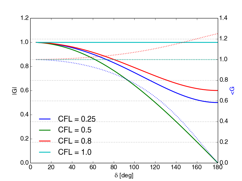
Figures 109 and 111 show (8.37) and (8.38) as a function of $ \delta $ for different values of the Courant-number. The range for which $ \varepsilon_D $ is close to 1 is larger than in Figure 109 for the upwind scheme. This puts in evidence an important difference between first and second order schemes Figure 110 shows that $ \varepsilon_\phi $ is generally less than 1, so that the numerical propagation speed is smaller than the physical one. This is the reason for the occurrence of oscillations as the ones shown in animation mov:step_movie. A von Neumann criterion guarantees stability for $ |G|\leq1 $, but does not guarantees that the scheme is monotone. On the other hand, the PC criterion ensures that no oscillations can occur. In fact, this criterion can not be verified for the Lax-Wendroff scheme applied to the linear advection equation. In fact, monotone schemes for the linear advection equation can be at most first order accurate.

Figure 109: Diffusion error $ \varepsilon_D $ (left y-axis) and dispersion error $ \varepsilon_\phi $ (right y-axis) as a function of frequency for the Lax-Wendroff scheme. The dotted lines of $ \varepsilon_\phi $ correspond to same CFL-numbers as solid lines of $ \varepsilon_D $ with the same color.

Figure 110: Dispersion error $ \varepsilon_\phi $ as a function of frequency for the Lax-Wendroff scheme.

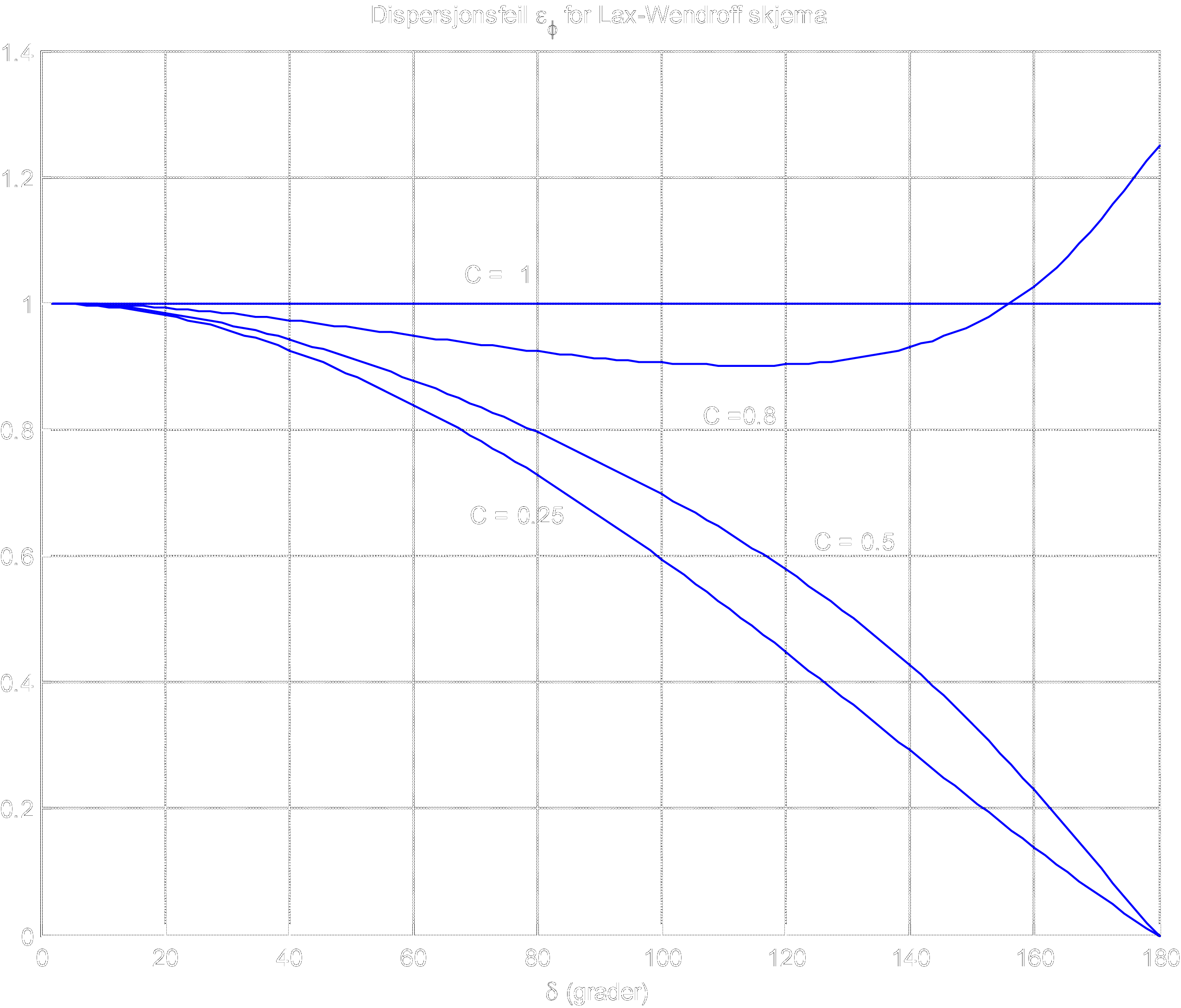
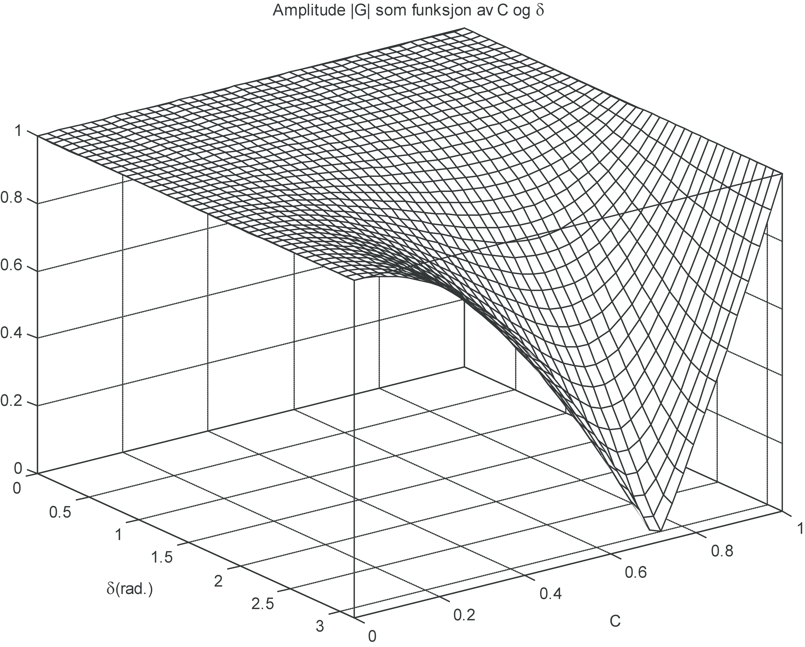
Figure 111: Diffusion error $ \varepsilon_D $ as a function of frequency and Courant-number for the Lax-Wendroff scheme.

8.6 The Lax-Friedrich Scheme

The Lax-Friedrich scheme is an explicit, first order scheme, using forward difference in time and central difference in space. However, the scheme is stabilized by averaging $ u^n_j $ over the neighbour cells in the in the temporal approximation: $$ \begin{equation} \frac{u_j^{n+1}-\frac{1}{2}(u^n_{j+1}+u^n_{j-1})}{\Delta t} = -\frac{F^n_{j+1}-F^n_{j-1}}{2 \Delta x} \tag{8.39} \end{equation} $$ The Lax-Friedrich scheme is the obtained by isolation $ u^{n+1}_j $ at the right hand side: $$ \begin{equation} u_j^{n+1} = \frac{1}{2}(u^n_{j+1}+u^n_{j-1}) - \frac{\Delta t}{2 \Delta x}(F^n_{j+1}-F^n_{j-1}) \label{} \end{equation} $$

By assuming a linear flux $ F=a_0 \, u $ it may be shown that the Lax-Friedrich scheme takes the form: $$ \begin{equation} u_j^{n+1} = \frac{1}{2}(u^n_{j+1}+u^n_{j-1}) - \frac{C}{2}(u^n_{j+1}-u^n_{j-1}) \tag{8.40} \end{equation} $$ where we have introduced the CFL-number as given by (8.6) and have the simple python-implementation:

def lax_friedrich(u):
    u[1:-1] = (u[:-2] +u[2:])/2.0 -  c*(u[2:] - u[:-2])/2.0
    return u[1:-1]

whereas a more generic flux implementation is implemented as:

def lax_friedrich_Flux(u):
    u[1:-1] = (u[:-2] +u[2:])/2.0 -  dt*(F(u[2:])-F(u[:-2]))/(2.0*dx)
    return u[1:-1]