2.16 Exercises
Exercise 1: Solving Newton's first differential equation using euler's method
One of the earliest known differential equations, which Newton solved with series expansion in 1671 is: $$ \begin{align} y'(x) =1-3x+y+x^2+xy,\ y(0)=0 \tag{2.164} \end{align} $$
Newton gave the following solution: $$ \begin{align} y(x) \approx x-x^2+\frac{x^3}{3}-\frac{x^4}{6}+ \frac{x^5}{30}-\frac{x^6}{45} \tag{2.165} \end{align} $$
Today it is possible to give the solution on closed form with known functions as follows, $$ \begin{align} y(x)=&3\sqrt{2\pi e}\cdot \exp\left[x\left(1+\frac{x}{2}\right)\right]\cdot \left[\text{erf}\left(\frac{\sqrt{2}}{2}(1+x)\right)-\text{erf}\left(\frac{\sqrt{2}}{2}\right)\right] + 4\cdot\left[1-\exp[x\left(1+\frac{x}{2}\right)\right]-x \tag{2.166} \end{align} $$
Note the combination \( \sqrt{2\pi e} \).
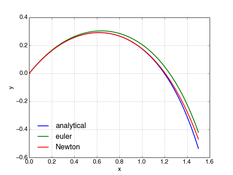
a) Solve equation (2.164) using Euler's method. Plot and compare with Newton's solution equation (2.165) and the analytical solution equation (2.166). Plot between \( x=0 \) and \( x=1.5 \)
The function scipy.special.erf will be needed. See http://docs.scipy.org/doc/scipy-0.15.1/reference/generated/scipy.special.erf.html.
Figure should look something like this:
Figure 25: Problem 1 with 101 samplepoints between \( x=0 \) and \( x=1.5 \) .
Exercise 2: Solitary wave
Figure 26: Solitary wave.
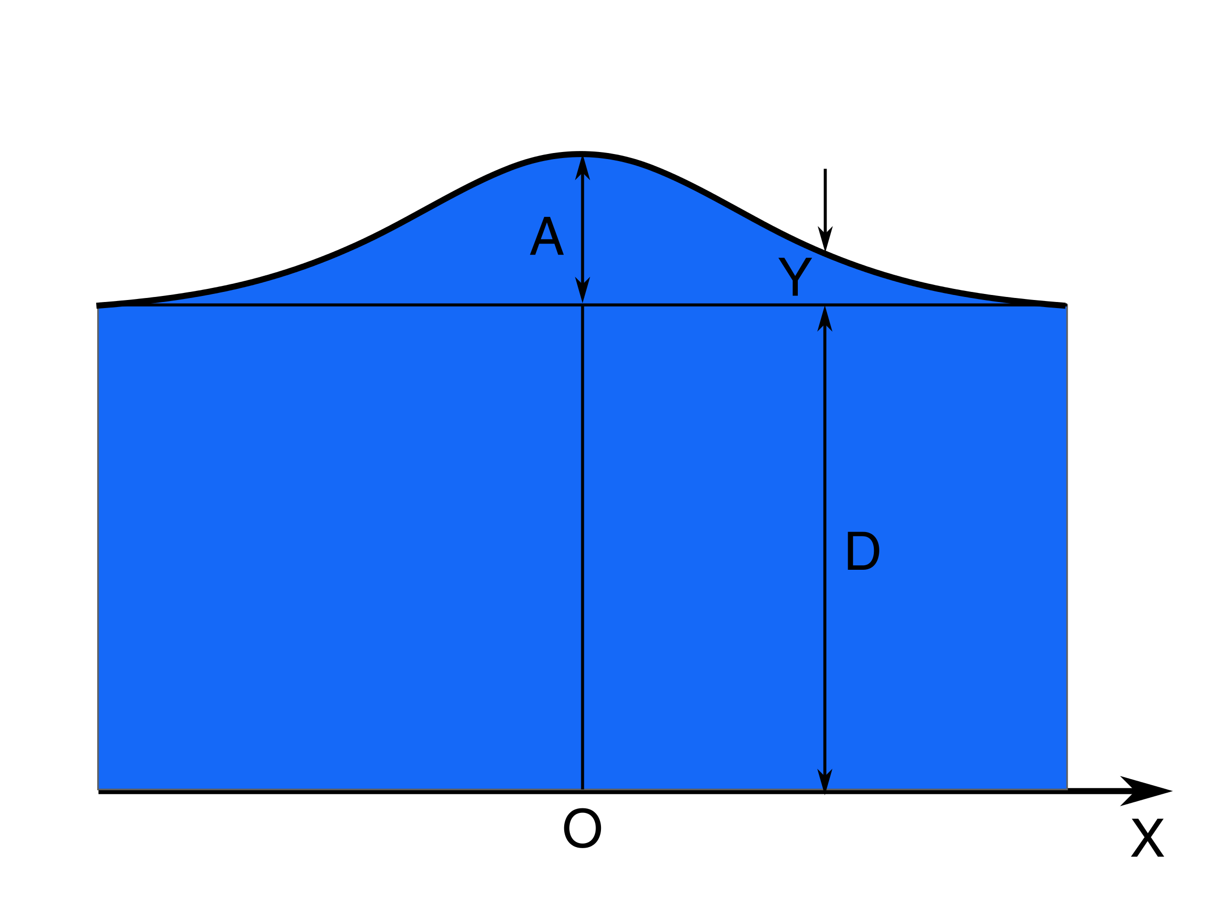
This exercise focuses on a solitary wave propagating on water. (PDF-version)
The differential equation for a solitary wave can be written as: $$ \begin{align} \frac{d^2 Y}{d X^2} = \frac{3Y}{D^2}\left(\frac{A}{D}-\frac{3}{2D}Y\right) \tag{2.167} \end{align} $$
where \( D \) is the middle depth, \( Y(X) \) is the wave height above middle depth and A is the wave height at \( X=0 \). The wave is symmetric with respect to \( X=0 \). See Figure 26. The coordinate system follows the wave.
By using dimensionless variables: \( x=\frac{X}{D} \), \( a=\frac{A}{D} \), \( y=\frac{Y}{A} \), equation (2.167) can be written as: $$ \begin{align} y''(x)=a \, 3 \, y(x) \, \left(1 - \frac{3}{2}y(x) \right) \tag{2.168} \end{align} $$
initial conditions: \( y(0)=1 \), \( y'(0)=0 \). Use \( a=\frac{2}{3} \)
Pen and paper
The following problems should be done using pen and paper:
a) Calculate y(0.6), and y'(0.6) using euler's method with \( \Delta x = 0.2 \)
b) Solve a) using Heuns's method.
c) Perform a taylor expansion series around \( x=0 \) (include 3 parts) on equation (2.168), and compare results with a)
and b).
d) Solve equation (2.168) analytically for \( a=\frac{2}{3} \), given:
$$
\begin{align}
\int \frac{dy}{y \, \sqrt{1-y}} = -2 \, arctanh \left(\sqrt{1-y}\right)
\nonumber
\end{align}
$$
Compare with solutions in a), b) and c).
Programing: Write a program that solve a), b) and c) numerically, and compare with the analytical solution found in d). Solve first with \( \Delta x = 0.2 \), and experiment with different values.
Hints for both Pen and paper and Programming problems:
Solutions:
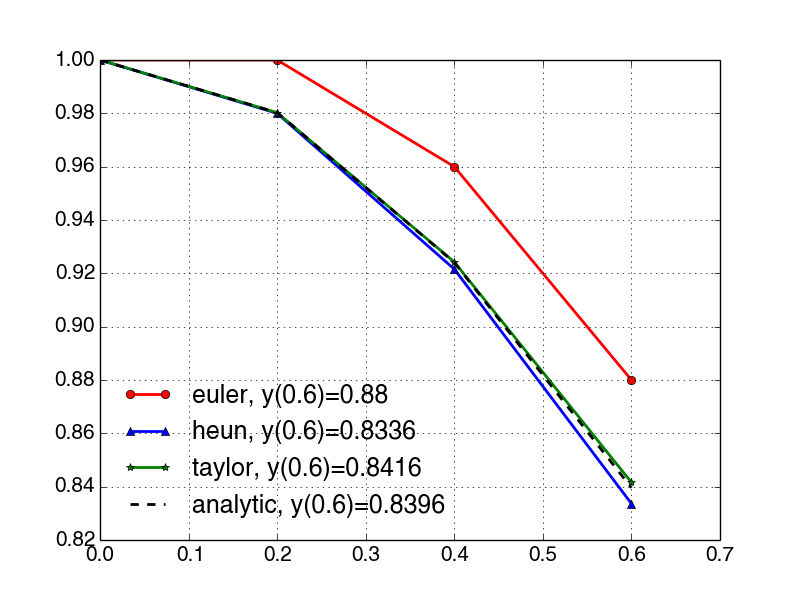
a) \( y(0.6)=0.88 \), \( y'(0.6)=-0.569 \).
b) \( y(0.6)=0.8337 \), \( y'(0.6)=-0.4858 \).
c) \( y \approx 1 - \frac{x^2}{2} + \frac{x^4}{6} \), \( y' \approx -x +\frac{2}{3}x^3 \)
d \( y = \frac{1}{cosh^2\left(x \, /\sqrt{2}\right)} = \frac{1}{1 + cosh\left(\sqrt{2} \cdot x\right)} \)
Figure 27: Plot should look something like this.
If you want you can use this template and fill in the lines where it's indicated.
# src-ch1/solitaryWave.py
#import matplotlib; matplotlib.use('Qt4Agg')
import matplotlib.pylab as plt
#plt.get_current_fig_manager().window.raise_()
import numpy as np

#### set default plot values: ####
LNWDT=3; FNT=15
plt.rcParams['lines.linewidth'] = LNWDT; plt.rcParams['font.size'] = FNT

""" This script solves the problem with the solitary wave:

        y'' = a*3*y*(1-y*3/2)

        y(0) = 1, y'(0) = 0

    or as a system of first order differential equations (y0 = y, y1 = y'):

        y0' = y'
        y1' = a*3*y0*(1-y0*3/2)

        y0(0) = 1, y1(0) = 0

"""
a = 2./3
h = 0.2 # steplength dx
x_0, x_end = 0, 0.6

x = np.arange(x_0, x_end + h, h) # allocate x values

#### solution vectors: ####
Y0_euler = np.zeros_like(x) # array to store y values
Y1_euler = np.zeros_like(x) # array to store y' values

Y0_heun = np.zeros_like(x)
Y1_heun = np.zeros_like(x)

#### initial conditions: ####
Y0_euler[0] = 1 # y(0) = 1
Y1_euler[0] = 0 # y'(0) = 0

Y0_heun[0] = 1
Y1_heun[0] = 0


#### solve with euler's method ####

for n in range(len(x) - 1):
    y0_n = Y0_euler[n] # y at this timestep
    y1_n = Y1_euler[n] # y' at this timestep

    "Fill in lines below"
    f0 =
    f1 =
    "Fill in lines above"

    Y0_euler[n + 1] = y0_n + h*f0
    Y1_euler[n + 1] = y1_n + h*f1

#### solve with heun's method: ####

for n in range(len(x) - 1):
    y0_n = Y0_heun[n] # y0 at this timestep (y_n)
    y1_n = Y1_heun[n] # y1 at this timestep (y'_n)

    "Fill in lines below"
    f0 =
    f1 =

    y0_p =
    y1_p =

    f0_p =
    f1_p =
    "Fill in lines above"

    Y0_heun[n + 1] = y0_n + 0.5*h*(f0 + f0_p)
    Y1_heun[n + 1] = y1_n + 0.5*h*(f1 + f1_p)


Y0_taylor = 1 - x**2/2 + x**4/6
Y1_taylor = -x + (2./3)*x**3

Y0_analytic = 1./(np.cosh(x/np.sqrt(2))**2)


#### Print and plot solutions: ####

print "a) euler's method: y({0})={1}, y'({2})={3}".format(x_end, round(Y0_euler[-1], 4), x_end, round(Y1_euler[-1], 4))
print "b) heun's method: y({0})={1}, y'({2})={3}".format(x_end, round(Y0_heun[-1], 4), x_end, round(Y1_heun[-1], 4))
print "c) Taylor series: y({0})={1}, y'({2})={3}".format(x_end, round(Y0_taylor[-1], 4), x_end, round(Y1_taylor[-1], 4))
print "d) Analytical solution: y({0})={1}".format(x_end, round(Y0_analytic[-1], 4))

plt.figure()
plt.plot(x, Y0_euler, 'r-o')
plt.plot(x, Y0_heun, 'b-^')
plt.plot(x, Y0_taylor, 'g-*')
plt.plot(x, Y0_analytic, 'k--')

eulerLegend = 'euler, y({0})={1}'.format(x_end, round(Y0_euler[-1], 4))
heunLegend = 'heun, y({0})={1}'.format(x_end, round(Y0_heun[-1], 4))
taylorLegend = 'taylor, y({0})={1}'.format(x_end, round(Y0_taylor[-1], 4))
analyticLegend = 'analytic, y({0})={1}'.format(x_end, round(Y0_analytic[-1], 4))

plt.legend([eulerLegend, heunLegend, taylorLegend, analyticLegend], loc='best', frameon=False)
plt.show()
Exercise 3: Mathematical pendulum
Figure 28: Mathematical pendulum.

Figure 28 shows a mathematical pendulum where the motion is described by the following ODE: $$ \begin{align} \frac{d ^2\theta}{d\tau^2} + \frac{g}{l} \sin\theta &=0 \tag{2.169} \end{align} $$
with initial conditions $$ \begin{align} &\theta(0) =\theta_0 \tag{2.170}\\ &\frac{d \theta}{d\tau}(0)=\dot\theta_0 \tag{2.171} \end{align} $$
We introduce a dimensionless time \( t=\sqrt{\frac{g}{l}}t \) such that (2.169) may be written as $$ \begin{align} \ddot\theta(t) + \sin\theta(t) &=0 \tag{2.172} \end{align} $$
with initial conditions $$ \begin{align} &\theta(0) =\theta_0 \tag{2.173}\\ &\dot\theta(0)=\dot\theta_0 \tag{2.174} \end{align} $$
Assume that the pendulum wire is a massless rod, such that \( -\pi \leq \theta_0 \leq \pi \).
The total energy (potential + kinetic), which is constant, may be written in dimensionless form as $$ \begin{align} \frac{1}{2}(\dot\theta)^2 - \cos\theta &= \frac{1}{2}(\dot\theta_0)^2 - \cos\theta_0 \tag{2.175} \end{align} $$ We define an energy function \( E(\theta) \) from (2.175) as $$ \begin{align} E(\theta) &= \frac{1}{2} [(\dot\theta)^2 - (\dot\theta_0)^2] + \cos\theta_0 - \cos\theta \tag{2.176} \end{align} $$ We see that this function should be identically equal to zero at all times. But, when it is computed numerically, it will deviate from zero due to numerical errors.
a) Write a Python program that solves the ODE in (2.172) with the specified initial conditions using Heun's method, for given values of \( \theta_0 \) and \( \dot\theta_0 \). Set for instance \( \theta_0=85^o \) and \( \dot\theta_0=0 \). (remember to convert use rad in ODE) Experiment with different time steps \( \Delta t \), and carry out the computation for at least a whole period. Plot both the amplitude and the energy function in (2.176) as functions of \( t \). Plot in separate figures.
b) Solve a) using Euler's method.
c) Solve the linearized version of the ODE in (2.172): $$ \begin{align} \tag{2.177} \ddot\theta (t)& + \theta (t) = 0 \\ \theta (0)& = \theta_0 ,\ \dot\theta (0) = 0 \tag{2.178} \end{align} $$
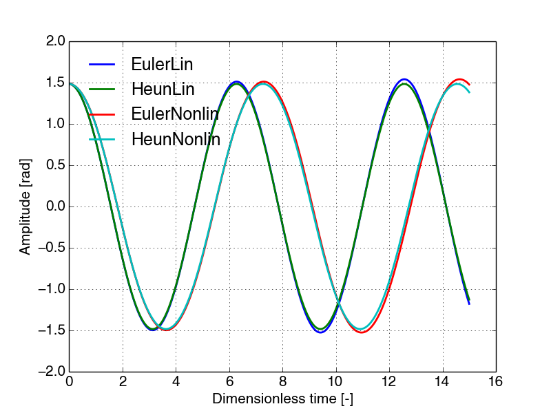
using both euler and Heuns method. Plot all four solutions (Problem 2, 3a and b) in the same figure. Experiment with different timesteps and values of \( \theta_0 \).
Euler implementations of the linearized version of this problem may be found in the digital compendium. See http://folk.ntnu.no/leifh/teaching/tkt4140/._main007.html.
Figure should look something like this:
Figure 29: Problem 3 with 2500 samplepoints and \( \theta_0 = 85^o \).
Exercise 4: Comparison of 2nd order RK-methods
In this exercise we seek to compare several 2nd order RK-methods as outlined in 2.10 Generic second order Runge-Kutta method.
a) Derive the Midpoint method \( a_2=1 \) and Ralston's method \( a_2=2/3 \) from the generic second order RK-method in (2.86).
b) Implement the Midpoint method \( a_2=1 \) and Ralston's method \( a_2=2/3 \) and compare their numerical predictions with the predictions of Heun's method for a model problem.