3.2 Shooting methods for boundary value problems with nonlinear ODEs
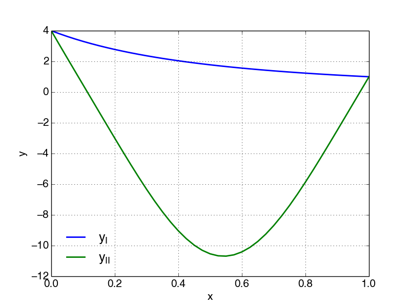
As model example for a non-linear boundary value problems we will investigate: $$ \begin{equation} \tag{3.59} \left.\begin{matrix} &y''(x)=\frac{3}{2}y^2 \\ &y(0)=4,\ y(1)=1 \end{matrix}\right.\ \end{equation} $$
Our model problem (3.59) may be proven to have two solutions.
- Solution I:
- Solution II:
- Can be expressed by elliptic Jacobi-functions ( see G.3 in Numeriske Beregninger)
Figure 37: The two solutions \( y_I \) and \( y_{II} \) of the non-linear ODE (3.59).
Our model equation (3.59) may be reduced to a system of ODEs in by introducing the common notation \( y\to y_0 \) and \( y'=y_0'=y_1 \) and following the procedure in 2.4 Reduction of Higher order Equations: $$ \begin{equation} \tag{3.61} \left.\begin{matrix} &y_0'(x)=y_1(x) \\ &y_1'(x)=\frac{3}{2}[y_0(x)]^2 \end{matrix}\right.\ \end{equation} $$
with the corresponding boundary conditions: $$ \begin{equation} y_0(0)=4,\ y_0(1)=1 \tag{3.62} \end{equation} $$
We will use the shooting method to find \( s=y'(0)=y_1(0) \) such that the boundary condition \( y_0(1)=1 \) is satisfied. Our boundary value error function becomes: $$ \begin{align} \phi (s^m)=y_0(1;s^m)-1,\ m=0,1,\dots \tag{3.63} \text{such that} \ y_0(1)\to 1 \ \text{for} \ \phi (s^m)\to0,\ m\to \infty \end{align} $$
As our model equation is non-linear our error function \( \phi(s) \) will also be non-linear, and we will have to conduct an iteration process as outlined in (3.63). Our task will then be to find the values \( s^* \) so that our boundary value error function \( \phi (s) \) becomes zero \( \phi (s^*)=0 \). For this purpose we choose the secant method (See [7], section 3.3).
Two initial guesses \( s^0 \) and \( s^1 \) are needed to start the iteration process. equation (3.61) is then solved twice (using \( s^0 \) and \( s^1 \)). From these solutions two values for the error function (3.63) may be calculated, namely \( \phi^0 \) and \( \phi^1 \). The next value of \( s \) (\( s^2 \)) is then found at the intersection of the gradient (calculated by the secant method) with the \( s-axis \).
For an arbitrary iteration, illustrated in Figure 38 we find it more convenient to introduce the \( \Delta s \): $$ \begin{equation} s^{m+1}=s^m+\Delta s \tag{3.64} \end{equation} $$
where $$ \begin{equation*} \Delta s=s^{m+1}-s^m=-\phi (s^m)\cdot \left[ \frac{s^m- s^{m-1}}{\phi (s^m)-\phi (s^{m-1})} \right],\ m=1,2,\dots \end{equation*} $$
Figure 38: An illustration of the usage of the secant method label to find the zero for a non-linear boundary value error function.

Given that \( s^{m-1} \) and \( s^m \) may be taken as known quantities the iteration process may be outlined as follows:
Examples on convergence criteria:
- Control of absolute error:
- Control of relative error:
The criteria (3.65) and (3.66) are frequently used in combination with: $$ \begin{equation} |\phi (s^{m+1})| < \varepsilon_3 \tag{3.67} \end{equation} $$
We will now use this iteration process to solve (3.61). However, a frequent problem is to find appropriate initial guesses, in particular in when \( \phi \) is a non-linear function and may have multiple solutions. A simple way to assess \( \phi \) is to make implement a program which plots \( \phi \) for a wide range of \( s \)-values and then vary this range until the zeros are in the range. An example for such a code is given below for our specific model problem:
# src-ch2/phi_plot_non_lin_ode.py;ODEschemes.py @ git@lrhgit/tkt4140/src/src-ch2/ODEschemes.py;

from ODEschemes import euler, heun, rk4
from numpy import cos, sin
import numpy as np
from matplotlib.pyplot import *

# change some default values to make plots more readable
LNWDT=2; FNT=11
rcParams['lines.linewidth'] = LNWDT; rcParams['font.size'] = FNT
font = {'size' : 16}; rc('font', **font)


N=20
L = 1.0
x = np.linspace(0,L,N+1)

def f(z, t):
    zout = np.zeros_like(z)
    zout[:] = [z[1],3.0*z[0]**2/2.0]
    return zout

beta=1.0 # Boundary value at x = L

solvers = [euler, heun, rk4] #list of solvers
solver=solvers[2] # select specific solver

smin=-45.0
smax=1.0
s_guesses = np.linspace(smin,smax,20)

# Guessed values
#s=[-5.0, 5.0]

z0=np.zeros(2)
z0[0] = 4.0

z = solver(f,z0,x)
phi0 = z[-1,0] - beta

nmax=10
eps = 1.0e-3
phi = []
for s in s_guesses:
    z0[1] = s
    z = solver(f,z0,x)
    phi.append(z[-1,0] - beta)


legends=[] # empty list to append legends as plots are generated

plot(s_guesses,phi)
ylabel('phi')
xlabel('s')
grid(b=True, which='both', color='0.65',linestyle='-')

show()
close()
Based on our plots of \( \phi \) we may now provided qualified initial guesses for and choose \( s^0=-3.0 \) and \( s^1=-6.0 \). The complete shooting method for the our boundary value problem may be found here:
# src-ch2/non_lin_ode.py;ODEschemes.py @ git@lrhgit/tkt4140/src/src-ch2/ODEschemes.py;

from ODEschemes import euler, heun, rk4
from numpy import cos, sin
import numpy as np
from matplotlib.pyplot import *

# change some default values to make plots more readable
LNWDT=3; FNT=16
rcParams['lines.linewidth'] = LNWDT; rcParams['font.size'] = FNT


N=40
L = 1.0
x = np.linspace(0,L,N+1)

def dsfunction(phi0,phi1,s0,s1):
    if (abs(phi1-phi0)>0.0):
        return    -phi1 *(s1 - s0)/float(phi1 - phi0)
    else:
        return 0.0


def f(z, t):
    zout = np.zeros_like(z)
    zout[:] = [z[1],3.0*z[0]**2/2.0]
    return zout


def y_analytical(x):
    return 4.0/(1.0+x)**2


beta=1.0 # Boundary value at x = L

solvers = [euler, heun, rk4] #list of solvers
solver=solvers[2] # select specific solver

# Guessed values
# s=[-3.0,-9]
s=[-40.0,-10.0]

z0=np.zeros(2)
z0[0] = 4.0
z0[1] = s[0]

z = solver(f,z0,x)
phi0 = z[-1,0] - beta

nmax=10
eps = 1.0e-3
for n in range(nmax):
    z0[1] = s[1]
    z = solver(f,z0,x)
    phi1 = z[-1,0] - beta
    ds = dsfunction(phi0,phi1,s[0],s[1])
    s[0]  = s[1]
    s[1] +=  ds
    phi0 = phi1
    print('n = {}  s1 = {} and ds = {}'.format(n,s[1],ds))

    if (abs(ds)<=eps):
        print('Solution converged for eps = {} and s1 ={} and ds = {}. \n'.format(eps,s[1],ds))
        break

legends=[] # empty list to append legends as plots are generated

plot(x,z[:,0])
legends.append('y')

plot(x,y_analytical(x),':^')
legends.append('y analytical')

# Add the labels
legend(legends,loc='best',frameon=False) # Add the legends
ylabel('y')
xlabel('x/L')
show()
After selection \( \Delta x=0.1 \) and using the RK4-solver, the following iteration output may be obtained:
| \( m \) | \( s^{m-1} \) | \( \phi (s^{m-1}) \) | \( s^m \) | \( \phi (s^m) \) | \( s^{m+1} \) | \( \phi (s^{m+1}) \) |
| 1 | -3.0 | 26.8131 | -6.0 | 6.2161 | -6.9054 | 2.9395 |
| 2 | -6.0 | 6.2161 | -6.9054 | 2.9395 | -7.7177 | 0.6697 |
| 3 | -6.9054 | 2.9395 | -7.7177 | 0.6697 | -7.9574 | 0.09875 |
| 4 | -7.7177 | 0.6697 | -7.9574 | 0.09875 | -7.9989 | 0.0004 |
After four iterations \( s=y'(0)= -7.9989 \) , while the analytical value is \( -8.0 \). The code \( non\_lin\_ode.py \) illustrates how our non-linear boundary value problem may be solve with a shooting method and offer graphical comparison of the numerical and analytical solution.
The secant method is simple and efficient and does not require any knowledge of the analytical expressions for the derivatives for the function for which the zeros are sought, like e.g. for Newton-Raphson's method. Clearly a drawback is that two initial guesses are mandatory to start the iteration process. However, by using some physical insight for the problem and plotting the \( \phi \)-function for a wide range of \( s \)-values, the problem is normally possible to deal with.