6.3.1 Neumann boundary conditions
Here we consider a heat conduction problem where we prescribe homogeneous Neuman boundary conditions, i.e. zero derivatives, at \( x=0 \) and \( y=0 \), as illustrated in figure 79.
Figure 79: Laplace-equation for a rectangular domain with homogeneous Neumann boundary conditions for \( x=0 \) and \( y=0 \).

Mathematically the problem in Figure 79, is specified with the governing equation (6.18) which we reiterate for convenience: $$ \begin{equation} \frac{\partial^2T}{\partial x^2}+\frac{\partial^2T}{\partial y^2}=0 \tag{6.27} \end{equation} $$ with homogeneous Neumann boundary conditions at: $$ \begin{align} \frac{\partial T}{\partial x}=0 \quad \text{ for } x=0, \text{ and } 0 < y < 1 \tag{6.28}\\ \frac{\partial T}{\partial y}=0 \quad \text{ for } y=0, \text{ and } 0 < x < 1 \tag{6.29} \end{align} $$ and prescribed values (Dirichlet boundary conditions) for: $$ \begin{align*} T=1 \quad \text{ for } y=1,\text{ and } 0\leq x\leq1\\ T=0 \quad \text{ for } x=1,\text{ and } 0\leq y < 1 \end{align*} $$
By assuming \( \Delta x=\Delta y \), as for the Dirichlet problem, an identical, generic difference equation is obtained as in (6.19). However, at the boundaries we need to take into account the Neumann boundary conditions. We will take a closer look at \( \dfrac{\partial T}{\partial x}=0 \) for \( x=0 \). The other Neumann boundary condition is treated in the same manner. Notice that we have discontinuities in the corners \( (1,0) \) and \( (1,1) \), additionally the corner \( (0,0) \) may cause problems too.
Figure 80: Illustration of how ghostcells with negative indices may be used to implement Neumann boundary conditions.

A central difference approximation (see Figure 80) of \( \dfrac{\partial T}{\partial x}=0 \) at \( i=0 \) yields: $$ \begin{equation} \frac{T_{1,j}-T_{-1,j}}{2\Delta x}=0 \to T_{-1,j}=T_{1,j} \tag{6.30} \end{equation} $$
where we have introduced ghostcells with negative indices outside the physical domain to express the derivative at the boundary. Note that the requirement of a zero derivative relate the value of the ghostcells to the values inside the physical domain.
One might also approximate \( \dfrac{\partial T}{\partial x}=0 \) by forward differences (see (6.16)) for a generic discrete point \( (i,j) \): $$ \begin{equation*} \frac{\partial T}{\partial x}\bigg|_ {i,j} = \frac{-3T_{i,j}+4T_{i+1,j}-T_{i+2,j}}{2\Delta x} \end{equation*} $$
which for \( \dfrac{\partial T}{\partial x}=0 \) for \( x=0 \) reduce to: $$ \begin{equation} T_{0,j}=\frac{4T_{1,j}-T_{2,j}}{3} \tag{6.31} \end{equation} $$
For the problem at hand, illustrated in Figure 79, central difference approximation (6.30) and forward difference approximation (6.31) yields fairly similar results, but (6.31) results in a shorter code when the methods in 6.4 Iterative methods for linear algebraic equation systems are employed.
To solve the problem in Figure 79 we employ the numerical stencil (6.20) for the unknowns in the field (not influenced by the boundaries) $$ \begin{equation} T_w+ T_e + T_s+ T_n -4 T_m=0 \tag{6.32} \end{equation} $$ where we used the same ordering as given in Figure 81. For the boundary conditions we have chosen to implement the by means of (6.30) which is illustrated in Figure 81 by the dashed lines.
Figure 81: Von Neumann boundary conditions with ghost cells.

Before setting up the complete equation system it normally pays of to look at the boundaries, like the lowermost boundary, which by systematic usage of (6.32) along with the boundary conditions in (6.29) yield: $$ \begin{align*} &2T_2+2T_5-4T_1=0\\ &T_1+2T_6+T_3-4T_2=0\\ &T_2+2T_7+T_4-4T_3=0\\ &T_3+2T_8-4T_4=0\\ \end{align*} $$ The equations for the upper boundary become: $$ \begin{align*} &T_9+2T_{14}-4T_{13}=-1\\ &T_{10}+T_{13}+T_{15}-4T_{14}=-1\\ &T_{11}+T_{14}+T_{16}-4T_{15}=-1\\ &T_{12}+T_{15}-4T_{16}=-1 \end{align*} $$
Notice that for the coarse mesh with only 16 unknown temperatures (see Figure 79) only 4 (\( T_{6} \), \( T_{7} \), \( T_{10} \), and \( T_{11} \)) are not explicitly influenced by the boundaries.Finally, the complete discretized equation system for the problem may be represented: $$ \begin{equation} \left(\begin{array}{cccccccccccccccc} -4& 2 & 0 & 0 & 2 & 0 & 0 & 0 & 0 & 0 & 0 & 0 & 0 & 0 &0 & 0\\ 1& -4 & 1 & 0 & 0 & 2 & 0 & 0 & 0 & 0 & 0 & 0 & 0 & 0 &0 & 0\\ 0& 1 & -4 & 1 & 0 & 0 & 2 & 0 & 0 & 0 & 0 & 0 & 0 & 0 &0 & 0\\ 0& 0 & 1 & -4 & 0 & 0 & 0 & 2 & 0 & 0 & 0 & 0 & 0 & 0 &0 & 0\\ 1& 0 & 0 & 0 & -4 & 2 & 0 & 0 & 1 & 0 & 0 & 0 & 0 & 0 &0 & 0\\ 0& 1 & 0 & 0 & 1 & -4 & 1 & 0 & 0 & 1 & 0 & 0 & 0 & 0 &0 & 0\\ 0& 0 & 1 & 0 & 0 & 1 & -4 & 1 & 0 & 0 & 1 & 0 & 0 & 0 &0 & 0\\ 0& 0 & 0 & 1 & 0 & 0 & 1 & -4 & 0 & 0 & 0 & 1 & 0 & 0 &0 & 0\\ 0& 0 & 0 & 0 & 1 & 0 & 0 & 0 & -4 & 2 & 0 & 0 & 1 & 0 &0 & 0\\ 0& 0 & 0 & 0 & 0 & 1 & 0 & 0 & 1 & -4 & 1 & 0 & 0 & 1 &0 & 0\\ 0& 0 & 0 & 0 & 0 & 0 &1 & 0 & 0 & 1 & -4 & 1 & 0 & 0 &1 & 0\\ 0& 0 & 0 & 0 & 0 & 0 & 0 & 1 & 0 & 0 & 1 & -4 & 0 & 0 &0 & 1\\ 0& 0 & 0 & 0 & 0 & 0 & 0 & 0 & 1 & 0 & 0 & 0 & -4 & 2 &0 & 0\\ 0& 0 & 0 & 0 & 0 & 0 & 0 & 0 & 0 & 1 & 0 & 0 & 1 & -4 &1 & 0\\ 0& 0 & 0 & 0 & 0 & 0 & 0 & 0 & 0 & 0 & 1 & 0 & 0 & 1 &-4 & 1\\ 0& 0 & 0 & 0 & 0 & 0 & 0 & 0 & 0 & 0 & 0 & 1 & 0 & 0 & 1 &-4 \end{array}\right) \cdot \left(\begin{array}{c} T_{1}\\ T_{2}\\ T_{3}\\ T_{4}\\ T_{5}\\ T_{6}\\ T_{7}\\ T_{8}\\ T_{9}\\ T_{10}\\ T_{11}\\ T_{12}\\ T_{13}\\ T_{14}\\ T_{15}\\ T_{16} \end{array}\right) = \left(\begin{array}{c} 0\\ 0\\ 0\\ 0\\ 0\\ 0\\ 0\\ 0\\ 0\\ 0\\ 0\\ 0\\ -1\\ -1\\ -1\\ -1 \end{array}\right) \tag{6.33} \end{equation} $$
# src-ch7/laplace_Neumann.py; Visualization.py @ git@lrhgit/tkt4140/src/src-ch7/Visualization.py;

import numpy as np
import scipy
import scipy.linalg
import scipy.sparse
import scipy.sparse.linalg
import matplotlib.pylab as plt
import time
from math import sinh

#import matplotlib.pyplot as plt

# Change some default values to make plots more readable on the screen
LNWDT=2; FNT=15
plt.rcParams['lines.linewidth'] = LNWDT; plt.rcParams['font.size'] = FNT

def setup_LaplaceNeumann_xy(Ttop, Tright, nx, ny):
    """ Function that returns A matrix and b vector  of the laplace Neumann heat problem A*T=b using central differences
        and assuming dx=dy, based on numbering with respect to x-dir, e.g:

                1   1   1             -4  2  2  0  0  0          0
            T6  T5  T6  0              1 -4  0  2  0  0          0
            T4  T3  T4  0              1  0 -4  2  1  0          0
            T2  T1  T2  0     --> A =  0  1  1 -4  0  1    ,b =  0
                T3  T4                 0  0  1  0 -4  2         -1
                                       0  0  0  1  1 -4         -1

            T = [T1, T2, T3, T4, T5, T6]^T

        Args:
            nx(int): number of elements in each row in the grid, nx=2 in the example above
            ny(int): number of elements in each column in the grid, ny=3 in the example above
        Returns:
            A(matrix): Sparse matrix A, in the equation A*T = b
            b(array): RHS, of the equation A*t = b
    """

    n = (nx)*(ny) #number of unknowns
    d = np.ones(n) # diagonals
    b = np.zeros(n) #RHS

    d0 = d.copy()*-4
    d1_lower = d.copy()[0:-1]
    d1_upper = d1_lower.copy()

    dnx_lower = d.copy()[0:-nx]
    dnx_upper = dnx_lower.copy()

    d1_lower[nx-1::nx] = 0 # every nx element on first diagonal is zero; starting from the nx-th element
    d1_upper[nx-1::nx] = 0
    d1_upper[::nx] = 2 # every nx element on first upper diagonal is two; stating from the first element.
                 # this correspond to all equations on border (x=0, y)

    dnx_upper[0:nx] = 2 # the first nx elements in the nx-th upper diagonal is two;
                        # This correspond to all equations on border (x, y=0)

    b[-nx:] = -Ttop
    b[nx-1::nx] += -Tright

    A = scipy.sparse.diags([d0, d1_upper, d1_lower, dnx_upper, dnx_lower], [0, 1, -1, nx, -nx], format='csc')

    return A, b

if __name__ == '__main__':
    from Visualization import plot_SurfaceNeumann_xy
    # Main program
    # Set temperature at the top
    Ttop=1
    Tright = 0.0
    xmax=1.0
    ymax=1.

    # Set simulation parameters
    #need hx=(1/nx)=hy=(1.5/ny)

    Nx = 10
    h=xmax/Nx
    Ny = int(ymax/h)

    A, b = setup_LaplaceNeumann_xy(Ttop, Tright, Nx, Ny)

    Temp = scipy.sparse.linalg.spsolve(A, b)

    plot_SurfaceNeumann_xy(Temp, Ttop, Tright, xmax, ymax, Nx, Ny)

#    figfile='LaPlace_vNeumann.png'
#    plt.savefig(figfile, format='png',transparent=True)
    plt.show()
The analytical solution is given by: $$ \begin{align} &T(x,y) = \sum^\infty_{n=1}A_n\cosh(\lambda_ny)\cdot\cos(\lambda_nx), \tag{6.34}\\ &\text{der } \lambda_n=(2n-1)\cdot\frac{\pi}{2},\ A_n=2\frac{(-1)^{n-1}}{\lambda_n\cosh(\lambda_n)},\ n=1,2,\dots \tag{6.35} \end{align} $$
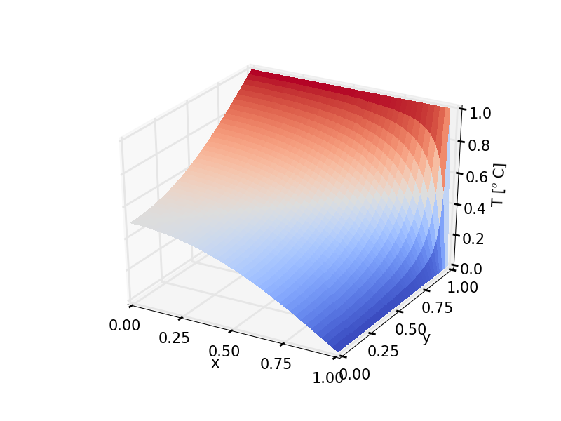
The solution for the problem illustrated Figure 79 is computed and visualized the python code above. The solution is illustrated in Figure 82.
Figure 82: Solution of the Laplace equation with Neuman boundary conditions.