3.1.1 Example: Couette-Poiseuille flow
In a Couette-Poiseuille flow, we consider fluid flow constrained between two walls, where the upper wall is moving at a prescribed velocity \( U_0 \) and at a distance \( Y=L \) from the bottom wall. Additionally, the flow is subjected to a prescribed pressure gradient \( \frac{\partial p}{\partial x} \).
Figure 32: An illustration of Couette flow driven by a pressure gradient and a moving upper wall.

We assume that the vertical velocity component \( V=0 \) and consequently we get from continuity: \( \frac{\partial U}{\partial X}=0 \) which implies that \( U=U(Y) \), i.e. the velocity in the streamwise X-direction depends on the cross-wise Y-direction only.
The equation of motion in the Y-direction simplifies to \( \frac{\partial p}{\partial Y}=-\rho g \), whereas the equation of motion in the X-direction has the form: $$ \begin{equation*} \rho U \cdot \frac{\partial U}{\partial X}=-\frac{\partial p}{\partial X} + \mu \left(\frac{\partial^2U}{\partial X^2}+ \frac{\partial^2U}{\partial Y^2}\right) \end{equation*} $$ which due to the above assumptions and ramifications reduces to $$ \begin{equation} \frac{d^2U}{dY^2} =\frac{1}{\mu}\frac{dp}{dX} \tag{3.20} \end{equation} $$
with no-slip boundary conditions: \( U(0)=0,\ U(L)=U_0 \). To render equation (3.20) on a more appropriate and generic form we introduce dimensionless variables: \( u=\frac{U}{U_0},\ y=\frac{Y}{L},\ P=-\frac{1}{U_0}(\frac{dp}{dX})\frac{L^2}{\mu} \), which yields: $$ \begin{equation} \frac{d^2u}{dy^2}=-P \tag{3.21} \end{equation} $$ with corresponding boundary conditions: $$ \begin{equation} u=0 \, \text{for} \, y=0, \qquad u=1 \, \text{for} \, y=1 \tag{3.22} \end{equation} $$
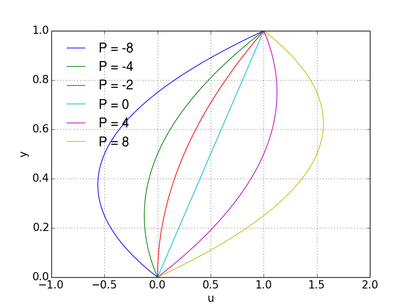
An analytical solution of equation (3.21) with the corresponding boundary conditions (3.22) may be found to be: $$ \begin{equation} u=y \cdot \left[ 1+\frac{P}{2}(1-y) \right] \tag{3.23} \end{equation} $$
Observe that for \( P\leq -2 \) we will get negative velocities for some values of \( y \). In Figure 33 velocity profiles are illustrated for a range of non-dimensional pressure gradients P.
Figure 33: Velocity profiles for Couette-Poiseuille flow with various pressure gradients.
To solve (3.21) numerically, we represent is as a system of equations: $$ \begin{equation} \left.\begin{matrix} &u'(y)=u_1(y) \\ &u_1'(y)=-P \end{matrix}\right.\ \tag{3.24} \end{equation} $$
with corresponding boundary conditions: $$ \begin{equation} u(0)=0,\ u(1)=1 \tag{3.25} \end{equation} $$
To solve this boundary value problem with a shooting method, we must find \( s=u'(0)=u_1(0) \) such that the boundary condition \( u(1)=1 \) is satisfied. We can express this condition by: $$ \begin{align*} \phi(s)=u(1;s)-1, \qquad \text{ such that } \qquad \phi(s)=0 & \qquad \text{when} \qquad s=s^* \end{align*} $$
We guess two values \( s^0 \) and \( s^1 \) and compute the correct \( s \) by linear interpolation due to the linearity of system of ODEs (3.24). For the linear interpolation see equation (3.14).
The shooting method is implemented in the python-code
Poiseuille_shoot.py and results are computed and plotted for a range
of non-dimensional pressure gradients and along with the analytical
solution.
# src-ch2/Couette_Poiseuille_shoot.py;ODEschemes.py @ git@lrhgit/tkt4140/src/src-ch2/ODEschemes.py;

from ODEschemes import euler, heun, rk4
import numpy as np
from matplotlib.pyplot import *

# change some default values to make plots more readable
LNWDT=5; FNT=11
rcParams['lines.linewidth'] = LNWDT; rcParams['font.size'] = FNT


N=200
L = 1.0
y = np.linspace(0,L,N+1)

def f(z, t):
    """RHS for Couette-Posieulle flow"""
    zout = np.zeros_like(z)
    zout[:] = [z[1], -dpdx]
    return zout

def u_a(y,dpdx):
    return y*(1.0 + dpdx*(1.0-y)/2.0);

beta=1.0 # Boundary value at y = L


# Guessed values
s=[1.0, 1.5]

z0=np.zeros(2)

dpdx_list=[-5.0, -2.5, -1.0, 0.0, 1.0,2.5, 5.0]
legends=[]

for dpdx in dpdx_list:
    phi = []
    for svalue in s:
        z0[1] = svalue
        z = rk4(f, z0, y)
        phi.append(z[-1,0] - beta)

    # Compute correct initial guess
    s_star = (s[0]*phi[1]-s[1]*phi[0])/(phi[1]-phi[0])
    z0[1] = s_star

    # Solve the initial value problem which is a solution to the boundary value problem
    z = rk4(f, z0, y)

    plot(z[:,0],y,'-.')
    legends.append('rk4: dp='+str(dpdx))

    # Plot the analytical solution
    plot(u_a(y, dpdx),y,':')
    legends.append('exa: dp='+str(dpdx))

# Add the labels
legend(legends,loc='best',frameon=False) # Add the legends
xlabel('u/U0')
ylabel('y/L')
show()