2.14 Numerical error as a function of \( \Delta t \) for ODE-schemes
To investigate whether the various ODE-schemes in our module 'ODEschemes.py' have the expected, theoretical order, we proceed in the same manner as outlined in (2.8.1 Example: Numerical error as a function of \( \Delta t \)). The complete code is listed at the end of this section but we will highlight and explain some details in the following.
To test the numerical order for the schemes we solve a somewhat general linear ODE: $$ \begin{align} \tag{2.125} u'(t)&= a \, u + b \\ u(t_0)&= u_0 \nonumber \end{align} $$ which has the analytical solutions: $$ \begin{equation} u =\begin{cases} \left (u_0 + \frac{b}{a} \right ) \; e^{a\, t} -\frac{b}{a},& \quad a \neq 0 \\ u_0 + b\, t, &\quad a = 0 \end{cases} \tag{2.126} \end{equation} $$
The right hand side defining the differential equation has been
implemented in function f3 and the corresponding
analytical solution is computed by u_nonlin_analytical:
    def f3(z, t, a=2.0, b=-1.0):
        """ """
        return a*z + b

    def u_nonlin_analytical(u0, t, a=2.0, b=-1.0):
        from numpy import exp
        TOL = 1E-14
        if (abs(a)>TOL):
            return (u0 + b/a)*exp(a*t)-b/a
        else:
            return u0 + b*t
The basic idea for the convergence test in the function
convergence_test is that we start out by
solving numerically an ODE with an analytical solution on a relatively
coarse grid, allowing for direct computations of the error. We then
reduce the timestep by a factor two (or double the grid size),
repeatedly, and compute the error for each grid and compare it with
the error of previous grid.
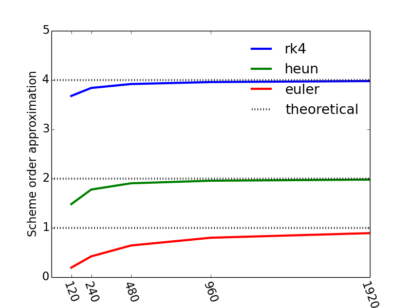
The Euler scheme (2.55) is \( O(h) \), whereas the Heun scheme (2.78) is \( O(h^2) \), and Runge-Kutta (2.96) is \( O(h^4) \), where the \( h \) denote a generic step size which for the current example is the timestep \( \Delta t \). The order of a particular scheme is given exponent \( n \) in the error term \( O(h^n) \). Consequently, the Euler scheme is a first oder scheme, Heun is second order, whereas Runge-Kutta is fourth order.
By letting \( \epsilon_{i+1} \) and \( \epsilon_i \) denote the errors on two consecutive grids with corresponding timesteps \( \displaystyle \Delta t_{i+1} = \frac{\Delta t_i}{2} \). The errors \( \epsilon_{i+1} \) and \( \epsilon_{i} \) for a scheme of order \( n \) are then related by: $$ \begin{equation} \tag{2.127} \epsilon_{i+1} = \frac{1}{2^n} \epsilon_{i} \end{equation} $$ Consequently, whenever \( \epsilon_{i+1} \) and \( \epsilon_{i} \) are known from consecutive simulations an estimate of the order of the scheme may be obtained by: $$ \begin{equation} \tag{2.128} n \approx \log_2 \frac{\epsilon_{i}}{\epsilon_{i+1}} \end{equation} $$ The theoretical value of \( n \) is thus \( n=1 \) for Euler's method, \( n=2 \) for Heun's method and \( n=4 \) for RK4.
In the function convergence_test the schemes we will subject to a
convergence test is ordered in a list scheme_list. This allows for a convenient loop over all schemes with the clause: for scheme in
scheme_list:. Subsequently, for each scheme we refine the initial
grid (N=30) Ndts times in the loop for i in range(Ndts+1): and
solve and compute the order estimate given by (2.128) with
the clause order_approx.append(previous_max_log_err -
max_log_err). Note that we can not compute this for the first
iteration (i=0), and that we use a an initial empty list
order_approx to store the approximation of the order n for each
grid refinement. For each grid we plot
\( \log_2(\epsilon) \) as a function of time with: plot(time[1:],
log_error, linestyles[i]+colors[iclr], markevery=N/5) and for each
plot we construct the corresponding legend by appending a new element
to the legends-list legends.append(scheme.func_name +': N = ' + str(N)). This construct produces a string with both the scheme name and the number of elements \( N \). The plot is not reproduced below, but you may see the result by downloading and running the module yourself.
Having completed the given number of refinements Ndts for a specific scheme
we store the order_approx for the scheme in a dictionary using the
name of the scheme as a key by schemes_orders[scheme.func_name] =
order_approx. This allows for an illustrative plot of the order estimate for each scheme with the clause:
for key in schemes_orders:
plot(N_list, (np.asarray(schemes_orders[key])))
and the resulting plot is shown in Figure 21, and we see that our numerical approximations for the orders of our schemes approach the theoretical values as the number of timesteps increase (or as the timestep is reduced by a factor two consecutively).
Figure 21: The convergence rate for the various ODE-solvers a function of the number of timesteps.
The complete function convergence_test is a part of the module ODEschemes and is isolated below:
def convergence_test():
""" Test convergence rate of the methods """
from numpy import linspace, size, abs, log10, mean, log2
figure()
tol = 1E-15
T = 8.0 # end of simulation
Ndts = 5 # Number of times to refine timestep in convergence test
z0 = 2
schemes =[euler, heun, rk4]
legends=[]
schemes_order={}
colors = ['r', 'g', 'b', 'm', 'k', 'y', 'c']
linestyles = ['-', '--', '-.', ':', 'v--', '*-.']
iclr = 0
for scheme in schemes:
N = 30 # no of time steps
time = linspace(0, T, N+1)
order_approx = []
for i in range(Ndts+1):
z = scheme(f3, z0, time)
abs_error = abs(u_nonlin_analytical(z0, time)-z[:,0])
log_error = log2(abs_error[1:]) # Drop 1st elt to avoid log2-problems (1st elt is zero)
max_log_err = max(log_error)
plot(time[1:], log_error, linestyles[i]+colors[iclr], markevery=N/5)
legends.append(scheme.__name__ +': N = ' + str(N))
# hold('on')
if i > 0: # Compute the log2 error difference
order_approx.append(previous_max_log_err -
max_log_err)
previous_max_log_err = max_log_err
N *=2
time = linspace(0, T, N+1)
schemes_order[scheme.__name__] = order_approx
iclr += 1
legend(legends, loc='best')
xlabel('Time')
ylabel('log(error)')
grid()
N = N/2**Ndts
N_list = [N*2**i for i in range(1, Ndts+1)]
N_list = np.asarray(N_list)
figure()
for key in schemes_order:
plot(N_list, (np.asarray(schemes_order[key])))
# Plot theoretical n for 1st, 2nd and 4th order schemes
axhline(1.0, xmin=0, xmax=N, linestyle=':', color='k')
axhline(2.0, xmin=0, xmax=N, linestyle=':', color='k')
axhline(4.0, xmin=0, xmax=N, linestyle=':', color='k')
xticks(N_list, rotation=-70)
legends = list(schemes_order.keys())
legends.append('theoretical')
legend(legends, loc='best', frameon=False)
xlabel('Number of unknowns')
ylabel('Scheme order approximation')
axis([0, max(N_list), 0, 5])
# savefig('ConvergenceODEschemes.png', transparent=True)
def manufactured_solution():
""" Test convergence rate of the methods, by using the Method of Manufactured solutions.
The coefficient function f is chosen to be the normal distribution
f = (1/(sigma*sqrt(2*pi)))*exp(-((t-mu)**2)/(2*sigma**2)).
The ODE to be solved is than chosen to be: f''' + f''*f + f' = RHS,
leading to to f''' = RHS - f''*f - f
"""
from numpy import linspace, size, abs, log10, mean, log2
from sympy import exp, symbols, diff, lambdify
from math import sqrt, pi
print("solving equation f''' + f''*f + f' = RHS")
print("which lead to f''' = RHS - f''*f - f")
t = symbols('t')
sigma=0.5 # standard deviation
mu=0.5 # mean value
Domain=[-1.5, 2.5]
t0 = Domain[0]
tend = Domain[1]
f = (1/(sigma*sqrt(2*pi)))*exp(-((t-mu)**2)/(2*sigma**2))
dfdt = diff(f, t)
d2fdt = diff(dfdt, t)
d3fdt = diff(d2fdt, t)
RHS = d3fdt + dfdt*d2fdt + f
f = lambdify([t], f)
dfdt = lambdify([t], dfdt)
d2fdt = lambdify([t], d2fdt)
RHS = lambdify([t], RHS)
def func(y,t):
yout = np.zeros_like(y)
yout[:] = [y[1], y[2], RHS(t) -y[0]- y[1]*y[2]]
return yout
z0 = np.array([f(t0), dfdt(t0), d2fdt(t0)])
figure()
tol = 1E-15
Ndts = 5 # Number of times to refine timestep in convergence test
schemes =[euler, heun, rk4]
legends=[]
schemes_order={}
colors = ['r', 'g', 'b', 'm', 'k', 'y', 'c']
linestyles = ['-', '--', '-.', ':', 'v--', '*-.']
iclr = 0
for scheme in schemes:
N = 100 # no of time steps
time = linspace(t0, tend, N+1)
fanalytic = np.zeros_like(time)
k = 0
for tau in time:
fanalytic[k] = f(tau)
k = k + 1
order_approx = []
for i in range(Ndts+1):
z = scheme(func, z0, time)
abs_error = abs(fanalytic-z[:,0])
log_error = log2(abs_error[1:]) # Drop 1st elt to avoid log2-problems (1st elt is zero)
max_log_err = max(log_error)
plot(time[1:],
log_error, linestyles[i]+colors[iclr], markevery=N/5)
legends.append(scheme.__name__ +': N = ' + str(N))
# hold('on')
if i > 0: # Compute the log2 error difference
order_approx.append(previous_max_log_err - max_log_err)
previous_max_log_err = max_log_err
N *=2
time = linspace(t0, tend, N+1)
fanalytic = np.zeros_like(time)
k = 0
for tau in time:
fanalytic[k] = f(tau)
k = k + 1
schemes_order[scheme.__name__] = order_approx
iclr += 1
legend(legends, loc='best')
xlabel('Time')
ylabel('log(error)')
grid()
N = N/2**Ndts
N_list = [N*2**i for i in range(1, Ndts+1)]
N_list = np.asarray(N_list)
figure()
for key in schemes_order:
plot(N_list, (np.asarray(schemes_order[key])))
# Plot theoretical n for 1st, 2nd and 4th order schemes
axhline(1.0, xmin=0, xmax=N, linestyle=':', color='k')
axhline(2.0, xmin=0, xmax=N, linestyle=':', color='k')
axhline(4.0, xmin=0, xmax=N, linestyle=':', color='k')
xticks(N_list, rotation=-70)
legends = list(schemes_order.keys())
legends.append('theoretical')
legend(legends, loc='best', frameon=False)
title('Method of Manufactured Solution')
xlabel('Number of unknowns')
ylabel('Scheme order approximation')
axis([0, max(N_list), 0, 5])
# savefig('MMSODEschemes.png', transparent=True)
# test using MMS and solving a set of two nonlinear equations to find estimate of order
def manufactured_solution_Nonlinear():
""" Test convergence rate of the methods, by using the Method of Manufactured solutions.
The coefficient function f is chosen to be the normal distribution
f = (1/(sigma*sqrt(2*pi)))*exp(-((t-mu)**2)/(2*sigma**2)).
The ODE to be solved is than chosen to be: f''' + f''*f + f' = RHS,
leading to f''' = RHS - f''*f - f
"""
from numpy import linspace, abs
from sympy import exp, symbols, diff, lambdify
from math import sqrt, pi
from numpy import log, log2
t = symbols('t')
sigma= 0.5 # standard deviation
mu = 0.5 # mean value
#### Perform needed differentiations based on the differential equation ####
f = (1/(sigma*sqrt(2*pi)))*exp(-((t-mu)**2)/(2*sigma**2))
dfdt = diff(f, t)
d2fdt = diff(dfdt, t)
d3fdt = diff(d2fdt, t)
RHS = d3fdt + dfdt*d2fdt + f
#### Create Python functions of f, RHS and needed differentiations of f ####
f = lambdify([t], f, np)
dfdt = lambdify([t], dfdt, np)
d2fdt = lambdify([t], d2fdt)
RHS = lambdify([t], RHS)
def func(y,t):
""" Function that returns the dfn/dt of the differential equation f + f''*f + f''' = RHS
as a system of 1st order equations; f = f1
f1' = f2
f2' = f3
f3' = RHS - f1 - f2*f3
Args:
y(array): solutian array [f1, f2, f3] at time t
t(float): current time
Returns:
yout(array): differantiation array [f1', f2', f3'] at time t
"""
yout = np.zeros_like(y)
yout[:] = [y[1], y[2], RHS(t) -y[0]- y[1]*y[2]]
return yout
t0, tend = -1.5, 2.5
z0 = np.array([f(t0), dfdt(t0), d2fdt(t0)]) # initial values
schemes = [euler, heun, rk4] # list of schemes; each of which is a function
schemes_error = {} # empty dictionary. to be filled in with lists of error-norms for all schemes
h = [] # empty list of time step
Ntds = 4 # number of times to refine dt
fig, ax = subplots(1, len(schemes), sharey = True, squeeze=False)
for k, scheme in enumerate(schemes):
N = 20 # initial number of time steps
error = [] # start of with empty list of errors for all schemes
legendList = []
for i in range(Ntds + 1):
time = linspace(t0, tend, N+1)
if k==0:
h.append(time[1] - time[0]) # add this iteration's dt to list h
z = scheme(func, z0, time) # Solve the ODE by calling the scheme with arguments. e.g: euler(func, z0, time)
fanalytic = f(time) # call analytic function f to compute analytical solutions at times: time
abs_error = abs(z[:,0]- fanalytic) # calculate infinity norm of the error
error.append(max(abs_error))
ax[0][k].plot(time, z[:,0])
legendList.append('$h$ = ' + str(h[i]))
N *=2 # refine dt
schemes_error[scheme.__name__] = error # Add a key:value pair to the dictionary. e.g: "euler":[error1, error2, ..., errorNtds]
ax[0][k].plot(time, fanalytic, 'k:')
legendList.append('$u_m$')
ax[0][k].set_title(scheme.__name__)
ax[0][k].set_xlabel('time')
ax[0][2].legend(legendList, loc = 'best', frameon=False)
ax[0][0].set_ylabel('u')
setp(ax, xticks=[-1.5, 0.5, 2.5], yticks=[0.0, 0.4 , 0.8, 1.2])
# #savefig('../figs/normal_distribution_refinement.png')
def Newton_solver_sympy(error, h, x0):
""" Function that solves for the nonlinear set of equations
error1 = C*h1^p --> f1 = C*h1^p - error1 = 0
error2 = C*h2^p --> f2 = C h2^p - error 2 = 0
where C is a constant h is the step length and p is the order,
with use of a newton rhapson solver. In this case C and p are
the unknowns, whereas h and error are knowns. The newton rhapson
method is an iterative solver which take the form:
xnew = xold - (J^-1)*F, where J is the Jacobi matrix and F is the
residual funcion.
x = [C, p]^T
J = [[df1/dx1 df2/dx2],
[df2/dx1 df2/dx2]]
F = [f1, f2]
This is very neatly done with use of the sympy module
Args:
error(list): list of calculated errors [error(h1), error(h2)]
h(list): list of steplengths corresponding to the list of errors
x0(list): list of starting (guessed) values for x
Returns:
x(array): iterated solution of x = [C, p]
"""
from sympy import Matrix
#### Symbolic computiations: ####
C, p = symbols('C p')
f1 = C*h[-2]**p - error[-2]
f2 = C*h[-1]**p - error[-1]
F = [f1, f2]
x = [C, p]
def jacobiElement(i,j):
return diff(F[i], x[j])
Jacobi = Matrix(2, 2, jacobiElement) # neat way of computing the Jacobi Matrix
JacobiInv = Jacobi.inv()
#### Numerical computations: ####
JacobiInvfunc = lambdify([x], JacobiInv)
Ffunc = lambdify([x], F)
x = x0
for n in range(8): #perform 8 iterations
F = np.asarray(Ffunc(x))
Jinv = np.asarray(JacobiInvfunc(x))
xnew = x - np.dot(Jinv, F)
x = xnew
#print "n, x: ", n, x
x[0] = round(x[0], 2)
x[1] = round(x[1], 3)
return x
ht = np.asarray(h)
eulerError = np.asarray(schemes_error["euler"])
heunError = np.asarray(schemes_error["heun"])
rk4Error = np.asarray(schemes_error["rk4"])
[C_euler, p_euler] = Newton_solver_sympy(eulerError, ht, [1,1])
[C_heun, p_heun] = Newton_solver_sympy(heunError, ht, [1,2])
[C_rk4, p_rk4] = Newton_solver_sympy(rk4Error, ht, [1,4])
from sympy import latex
h = symbols('h')
epsilon_euler = C_euler*h**p_euler
epsilon_euler_latex = '$' + latex(epsilon_euler) + '$'
epsilon_heun = C_heun*h**p_heun
epsilon_heun_latex = '$' + latex(epsilon_heun) + '$'
epsilon_rk4 = C_rk4*h**p_rk4
epsilon_rk4_latex = '$' + latex(epsilon_rk4) + '$'
print(epsilon_euler_latex)
print(epsilon_heun_latex)
print(epsilon_rk4_latex)
epsilon_euler = lambdify(h, epsilon_euler, np)
epsilon_heun = lambdify(h, epsilon_heun, np)
epsilon_rk4 = lambdify(h, epsilon_rk4, np)
N = N/2**(Ntds + 2)
N_list = [N*2**i for i in range(1, Ntds + 2)]
N_list = np.asarray(N_list)
print(len(N_list))
print(len(eulerError))
figure()
plot(N_list, log2(eulerError), 'b')
plot(N_list, log2(epsilon_euler(ht)), 'b--')
plot(N_list, log2(heunError), 'g')
plot(N_list, log2(epsilon_heun(ht)), 'g--')
plot(N_list, log2(rk4Error), 'r')
plot(N_list, log2(epsilon_rk4(ht)), 'r--')
LegendList = ['${\epsilon}_{euler}$', epsilon_euler_latex, '${\epsilon}_{heun}$', epsilon_heun_latex, '${\epsilon}_{rk4}$', epsilon_rk4_latex]
legend(LegendList, loc='best', frameon=False)
xlabel('-log(h)')
ylabel('-log($\epsilon$)')
# #savefig('../figs/MMS_example2.png')
The complete module ODEschemes is listed below and may easily be downloaded in your Eclipse/LiClipse IDE:
# src-ch1/ODEschemes.py
import numpy as np
from matplotlib.pyplot import plot, show, legend, rcParams,rc, figure, axhline, close,\
xticks, title, xlabel, ylabel, savefig, axis, grid, subplots, setp
# change some default values to make plots more readable
LNWDT=3; FNT=10
rcParams['lines.linewidth'] = LNWDT; rcParams['font.size'] = FNT
# define Euler solver
def euler(func, z0, time):
"""The Euler scheme for solution of systems of ODEs.
z0 is a vector for the initial conditions,
the right hand side of the system is represented by func which returns
a vector with the same size as z0 ."""
z = np.zeros((np.size(time), np.size(z0)))
z[0,:] = z0
for i in range(len(time)-1):
dt = time[i+1] - time[i]
z[i+1,:]=z[i,:] + np.asarray(func(z[i,:], time[i]))*dt
return z
# define Heun solver
def heun(func, z0, time):
"""The Heun scheme for solution of systems of ODEs.
z0 is a vector for the initial conditions,
the right hand side of the system is represented by func which returns
a vector with the same size as z0 ."""
z = np.zeros((np.size(time), np.size(z0)))
z[0,:] = z0
zp = np.zeros_like(z0)
for i, t in enumerate(time[0:-1]):
dt = time[i+1] - time[i]
zp = z[i,:] + np.asarray(func(z[i,:],t))*dt # Predictor step
z[i+1,:] = z[i,:] + (np.asarray(func(z[i,:],t)) + np.asarray(func(zp,t+dt)))*dt/2.0 # Corrector step
return z
# define rk4 scheme
def rk4(func, z0, time):
"""The Runge-Kutta 4 scheme for solution of systems of ODEs.
z0 is a vector for the initial conditions,
the right hand side of the system is represented by func which returns
a vector with the same size as z0 ."""
z = np.zeros((np.size(time),np.size(z0)))
z[0,:] = z0
zp = np.zeros_like(z0)
for i, t in enumerate(time[0:-1]):
dt = time[i+1] - time[i]
dt2 = dt/2.0
k1 = np.asarray(func(z[i,:], t)) # predictor step 1
k2 = np.asarray(func(z[i,:] + k1*dt2, t + dt2)) # predictor step 2
k3 = np.asarray(func(z[i,:] + k2*dt2, t + dt2)) # predictor step 3
k4 = np.asarray(func(z[i,:] + k3*dt, t + dt)) # predictor step 4
z[i+1,:] = z[i,:] + dt/6.0*(k1 + 2.0*k2 + 2.0*k3 + k4) # Corrector step
return z
if __name__ == '__main__':
a = 0.2
b = 3.0
u_exact = lambda t: a*t + b
def f_local(u,t):
"""A function which returns an np.array but less easy to read
than f(z,t) below. """
return np.asarray([a + (u - u_exact(t))**5])
def f(z, t):
"""Simple to read function implementation """
return [a + (z - u_exact(t))**5]
def test_ODEschemes():
"""Use knowledge of an exact numerical solution for testing."""
from numpy import linspace, size
tol = 1E-15
T = 2.0 # end of simulation
N = 20 # no of time steps
time = linspace(0, T, N+1)
z0 = np.zeros(1)
z0[0] = u_exact(0.0)
schemes = [euler, heun, rk4]
for scheme in schemes:
z = scheme(f, z0, time)
max_error = np.max(u_exact(time) - z[:,0])
msg = '%s failed with error = %g' % (scheme.__name__, max_error)
assert max_error < tol, msg
# f3 defines an ODE with analytical solution in u_nonlin_analytical
def f3(z, t, a=2.0, b=-1.0):
""" """
return a*z + b
def u_nonlin_analytical(u0, t, a=2.0, b=-1.0):
from numpy import exp
TOL = 1E-14
if (abs(a)>TOL):
return (u0 + b/a)*exp(a*t)-b/a
else:
return u0 + b*t
# Function for convergence test
    def convergence_test():
        """ Test convergence rate of the methods """
        from numpy import linspace, size, abs, log10, mean, log2
        figure()
        tol = 1E-15
        T = 8.0   # end of simulation
        Ndts = 5 # Number of times to refine timestep in convergence test

        z0 = 2

        schemes =[euler, heun, rk4]
        legends=[]
        schemes_order={}

        colors = ['r', 'g', 'b', 'm', 'k', 'y', 'c']
        linestyles = ['-', '--', '-.', ':', 'v--', '*-.']
        iclr = 0
        for scheme in schemes:
            N = 30    # no of time steps
            time = linspace(0, T, N+1)

            order_approx = []

            for i in range(Ndts+1):
                z = scheme(f3, z0, time)
                abs_error = abs(u_nonlin_analytical(z0, time)-z[:,0])
                log_error = log2(abs_error[1:]) # Drop 1st elt to avoid log2-problems (1st elt is zero)
                max_log_err = max(log_error)
                plot(time[1:], log_error, linestyles[i]+colors[iclr], markevery=N/5)
                legends.append(scheme.__name__ +': N = ' + str(N))
#                hold('on')

                if i > 0: # Compute the log2 error difference
                    order_approx.append(previous_max_log_err - max_log_err)
                previous_max_log_err = max_log_err

                N *=2
                time = linspace(0, T, N+1)

            schemes_order[scheme.__name__] = order_approx
            iclr += 1

        legend(legends, loc='best')
        xlabel('Time')
        ylabel('log(error)')
        grid()

        N = N/2**Ndts
        N_list = [N*2**i for i in range(1, Ndts+1)]
        N_list = np.asarray(N_list)

        figure()
        for key in schemes_order:
            plot(N_list, (np.asarray(schemes_order[key])))

        # Plot theoretical n for 1st, 2nd and 4th order schemes
        axhline(1.0, xmin=0, xmax=N, linestyle=':', color='k')
        axhline(2.0, xmin=0, xmax=N, linestyle=':', color='k')
        axhline(4.0, xmin=0, xmax=N, linestyle=':', color='k')
        xticks(N_list, rotation=-70)
        legends = list(schemes_order.keys())
        legends.append('theoretical')
        legend(legends, loc='best', frameon=False)
        xlabel('Number of unknowns')
        ylabel('Scheme order approximation')
        axis([0, max(N_list), 0, 5])
#        savefig('ConvergenceODEschemes.png', transparent=True)

    def manufactured_solution():
        """ Test convergence rate of the methods, by using the Method of Manufactured solutions.
            The coefficient function f is chosen to be the normal distribution
            f = (1/(sigma*sqrt(2*pi)))*exp(-((t-mu)**2)/(2*sigma**2)).
            The ODE to be solved is than chosen to be: f''' + f''*f + f' = RHS,
            leading to to f''' = RHS - f''*f - f
         """
        from numpy import linspace, size, abs, log10, mean, log2
        from sympy import exp, symbols, diff, lambdify
        from math import sqrt, pi

        print("solving equation f''' + f''*f + f' = RHS")
        print("which lead to f''' = RHS - f''*f - f")
        t = symbols('t')
        sigma=0.5 # standard deviation
        mu=0.5 # mean value
        Domain=[-1.5, 2.5]
        t0 = Domain[0]
        tend = Domain[1]

        f = (1/(sigma*sqrt(2*pi)))*exp(-((t-mu)**2)/(2*sigma**2))
        dfdt = diff(f, t)
        d2fdt = diff(dfdt, t)
        d3fdt = diff(d2fdt, t)
        RHS = d3fdt + dfdt*d2fdt + f

        f = lambdify([t], f)
        dfdt = lambdify([t], dfdt)
        d2fdt = lambdify([t], d2fdt)
        RHS = lambdify([t], RHS)

        def func(y,t):
            yout = np.zeros_like(y)
            yout[:] = [y[1], y[2], RHS(t) -y[0]- y[1]*y[2]]

            return yout

        z0 = np.array([f(t0), dfdt(t0), d2fdt(t0)])

        figure()
        tol = 1E-15
        Ndts = 5 # Number of times to refine timestep in convergence test
        schemes =[euler, heun, rk4]
        legends=[]
        schemes_order={}

        colors = ['r', 'g', 'b', 'm', 'k', 'y', 'c']
        linestyles = ['-', '--', '-.', ':', 'v--', '*-.']
        iclr = 0
        for scheme in schemes:
            N = 100    # no of time steps
            time = linspace(t0, tend, N+1)
            fanalytic = np.zeros_like(time)
            k = 0
            for tau in time:
                fanalytic[k] = f(tau)
                k = k + 1

            order_approx = []

            for i in range(Ndts+1):
                z = scheme(func, z0, time)
                abs_error = abs(fanalytic-z[:,0])
                log_error = log2(abs_error[1:]) # Drop 1st elt to avoid log2-problems (1st elt is zero)
                max_log_err = max(log_error)
                plot(time[1:], log_error, linestyles[i]+colors[iclr], markevery=N/5)
                legends.append(scheme.__name__ +': N = ' + str(N))
#                hold('on')

                if i > 0: # Compute the log2 error difference
                    order_approx.append(previous_max_log_err - max_log_err)
                previous_max_log_err = max_log_err

                N *=2
                time = linspace(t0, tend, N+1)
                fanalytic = np.zeros_like(time)
                k = 0
                for tau in time:
                    fanalytic[k] = f(tau)
                    k = k + 1

            schemes_order[scheme.__name__] = order_approx
            iclr += 1

        legend(legends, loc='best')
        xlabel('Time')
        ylabel('log(error)')
        grid()

        N = N/2**Ndts
        N_list = [N*2**i for i in range(1, Ndts+1)]
        N_list = np.asarray(N_list)

        figure()
        for key in schemes_order:
            plot(N_list, (np.asarray(schemes_order[key])))

        # Plot theoretical n for 1st, 2nd and 4th order schemes
        axhline(1.0, xmin=0, xmax=N, linestyle=':', color='k')
        axhline(2.0, xmin=0, xmax=N, linestyle=':', color='k')
        axhline(4.0, xmin=0, xmax=N, linestyle=':', color='k')
        xticks(N_list, rotation=-70)
        legends = list(schemes_order.keys())
        legends.append('theoretical')
        legend(legends, loc='best', frameon=False)
        title('Method of Manufactured Solution')
        xlabel('Number of unknowns')
        ylabel('Scheme order approximation')
        axis([0, max(N_list), 0, 5])
#        savefig('MMSODEschemes.png', transparent=True)
    # test using MMS and solving a set of two nonlinear equations to find estimate of order
    def manufactured_solution_Nonlinear():
        """ Test convergence rate of the methods, by using the Method of Manufactured solutions.
            The coefficient function f is chosen to be the normal distribution
            f = (1/(sigma*sqrt(2*pi)))*exp(-((t-mu)**2)/(2*sigma**2)).
            The ODE to be solved is than chosen to be: f''' + f''*f + f' = RHS,
            leading to f''' = RHS - f''*f - f
         """
        from numpy import linspace, abs
        from sympy import exp, symbols, diff, lambdify
        from math import sqrt, pi
        from numpy import log, log2

        t = symbols('t')
        sigma=  0.5 # standard deviation
        mu = 0.5 # mean value
        #### Perform needed differentiations based on the differential equation ####
        f = (1/(sigma*sqrt(2*pi)))*exp(-((t-mu)**2)/(2*sigma**2))
        dfdt = diff(f, t)
        d2fdt = diff(dfdt, t)
        d3fdt = diff(d2fdt, t)
        RHS = d3fdt + dfdt*d2fdt + f
        #### Create Python functions of f, RHS and needed differentiations of f ####
        f = lambdify([t], f, np)
        dfdt = lambdify([t], dfdt, np)
        d2fdt = lambdify([t], d2fdt)
        RHS = lambdify([t], RHS)

        def func(y,t):
            """ Function that returns the dfn/dt of the differential equation f + f''*f + f''' = RHS
                as a system of 1st order equations; f = f1
                        f1' = f2
                        f2' = f3
                        f3' = RHS - f1 - f2*f3

                Args:
                    y(array): solutian array [f1, f2, f3] at time t
                    t(float): current time

                Returns:
                    yout(array): differantiation array [f1', f2', f3'] at time t
            """
            yout = np.zeros_like(y)
            yout[:] = [y[1], y[2], RHS(t) -y[0]- y[1]*y[2]]

            return yout

        t0, tend = -1.5, 2.5
        z0 = np.array([f(t0), dfdt(t0), d2fdt(t0)]) # initial values

        schemes = [euler, heun, rk4] # list of schemes; each of which is a function
        schemes_error = {} # empty dictionary. to be filled in with lists of error-norms for all schemes
        h = [] # empty list of time step

        Ntds = 4 # number of times to refine dt

        fig, ax = subplots(1, len(schemes), sharey = True, squeeze=False)

        for k, scheme in enumerate(schemes):
            N = 20    # initial number of time steps
            error = [] # start of with empty list of errors for all schemes
            legendList = []

            for i in range(Ntds + 1):
                time = linspace(t0, tend, N+1)

                if k==0:
                    h.append(time[1] - time[0]) # add this iteration's dt to list h
                z = scheme(func, z0, time) # Solve the ODE by calling the scheme with arguments. e.g: euler(func, z0, time)
                fanalytic = f(time) # call analytic function f to compute analytical solutions at times: time

                abs_error = abs(z[:,0]- fanalytic) # calculate infinity norm of the error
                error.append(max(abs_error))

                ax[0][k].plot(time, z[:,0])
                legendList.append('$h$ = ' + str(h[i]))

                N *=2 # refine dt

            schemes_error[scheme.__name__] = error # Add a key:value pair to the dictionary. e.g: "euler":[error1, error2, ..., errorNtds]


            ax[0][k].plot(time, fanalytic, 'k:')
            legendList.append('$u_m$')
            ax[0][k].set_title(scheme.__name__)
            ax[0][k].set_xlabel('time')

        ax[0][2].legend(legendList, loc = 'best', frameon=False)
        ax[0][0].set_ylabel('u')
        setp(ax, xticks=[-1.5, 0.5,  2.5], yticks=[0.0, 0.4 , 0.8, 1.2])

#        #savefig('../figs/normal_distribution_refinement.png')
        def Newton_solver_sympy(error, h, x0):
            """ Function that solves for the nonlinear set of equations
                error1 = C*h1^p --> f1 = C*h1^p - error1 = 0
                error2 = C*h2^p --> f2 = C h2^p - error 2 = 0
                where C is a constant h is the step length and p is the order,
                with use of a newton rhapson solver. In this case C and p are
                the unknowns, whereas h and error are knowns. The newton rhapson
                method is an iterative solver which take the form:
                xnew = xold - (J^-1)*F, where J is the Jacobi matrix and F is the
                residual funcion.
                    x = [C, p]^T
                    J = [[df1/dx1  df2/dx2],
                         [df2/dx1  df2/dx2]]
                    F = [f1, f2]
                This is very neatly done with use of the sympy module

                Args:
                    error(list): list of calculated errors [error(h1), error(h2)]
                    h(list): list of steplengths corresponding to the list of errors
                    x0(list): list of starting (guessed) values for x

                Returns:
                    x(array): iterated solution of x = [C, p]

            """
            from sympy import Matrix
            #### Symbolic computiations: ####
            C, p = symbols('C p')
            f1 = C*h[-2]**p - error[-2]
            f2 = C*h[-1]**p - error[-1]
            F = [f1, f2]
            x = [C, p]

            def jacobiElement(i,j):
                return diff(F[i], x[j])

            Jacobi = Matrix(2, 2, jacobiElement) # neat way of computing the Jacobi Matrix
            JacobiInv = Jacobi.inv()
            #### Numerical computations: ####
            JacobiInvfunc = lambdify([x], JacobiInv)
            Ffunc = lambdify([x], F)
            x = x0

            for n in range(8): #perform 8 iterations
                F = np.asarray(Ffunc(x))
                Jinv = np.asarray(JacobiInvfunc(x))
                xnew = x - np.dot(Jinv, F)
                x = xnew
                #print "n, x: ", n, x
            x[0] = round(x[0], 2)
            x[1] = round(x[1], 3)
            return x

        ht = np.asarray(h)
        eulerError = np.asarray(schemes_error["euler"])
        heunError = np.asarray(schemes_error["heun"])
        rk4Error = np.asarray(schemes_error["rk4"])


        [C_euler, p_euler] = Newton_solver_sympy(eulerError, ht, [1,1])
        [C_heun, p_heun] = Newton_solver_sympy(heunError, ht, [1,2])
        [C_rk4, p_rk4] = Newton_solver_sympy(rk4Error, ht, [1,4])

        from sympy import latex
        h = symbols('h')
        epsilon_euler = C_euler*h**p_euler
        epsilon_euler_latex = '$' + latex(epsilon_euler) + '$'
        epsilon_heun = C_heun*h**p_heun
        epsilon_heun_latex = '$' + latex(epsilon_heun) + '$'
        epsilon_rk4 = C_rk4*h**p_rk4
        epsilon_rk4_latex = '$' + latex(epsilon_rk4) + '$'

        print(epsilon_euler_latex)
        print(epsilon_heun_latex)
        print(epsilon_rk4_latex)

        epsilon_euler = lambdify(h, epsilon_euler, np)
        epsilon_heun = lambdify(h, epsilon_heun, np)
        epsilon_rk4 = lambdify(h, epsilon_rk4, np)

        N = N/2**(Ntds + 2)
        N_list = [N*2**i for i in range(1, Ntds + 2)]
        N_list = np.asarray(N_list)
        print(len(N_list))
        print(len(eulerError))
        figure()
        plot(N_list, log2(eulerError), 'b')
        plot(N_list, log2(epsilon_euler(ht)), 'b--')
        plot(N_list, log2(heunError), 'g')
        plot(N_list, log2(epsilon_heun(ht)), 'g--')
        plot(N_list, log2(rk4Error), 'r')
        plot(N_list, log2(epsilon_rk4(ht)), 'r--')
        LegendList = ['${\epsilon}_{euler}$', epsilon_euler_latex, '${\epsilon}_{heun}$', epsilon_heun_latex, '${\epsilon}_{rk4}$', epsilon_rk4_latex]
        legend(LegendList, loc='best', frameon=False)
        xlabel('-log(h)')
        ylabel('-log($\epsilon$)')

#        #savefig('../figs/MMS_example2.png')
def plot_ODEschemes_solutions():
"""Plot the solutions for the test schemes in schemes"""
from numpy import linspace
figure()
T = 1.5 # end of simulation
N = 50 # no of time steps
time = linspace(0, T, N+1)
z0 = 2.0
schemes = [euler, heun, rk4]
legends = []
for scheme in schemes:
z = scheme(f3, z0, time)
plot(time, z[:,-1])
legends.append(scheme.__name__)
plot(time, u_nonlin_analytical(z0, time))
legends.append('analytical')
legend(legends, loc='best', frameon=False)
manufactured_solution_Nonlinear()
#test_ODEschemes()
#convergence_test()
#plot_ODEschemes_solutions()
#manufactured_solution()
show()