• «
• 1
• ...
• 48
• 49
• 50
• 51
• 52
• 53
• 54
• 55
• 56
• 57
• 58
• 59
• 60
• 61
• 62
• 63
• 64
• 65
• ...
• 79
• »

6.2 Finite differences. Notation

In the section 2.5 Differences we used Taylor expansions to discretize differential equations for functions of one independent variable. A similar procedure can be applied to functions of more than one independent variable In particular, if the expressions to be discretized have no cross-derivatives, we can apply the formulas derived in the section 2.5 Differences, keeping the index for the second variable constant.

Since we are dealing with elliptic equations, we will, for convenience, consider \( x \) and \( y \) as the independent variables. Moreover, its discretization is given by: $$ \begin{align*} &x_i=x_0+i\cdot \Delta x,\ i=0,1,2,\dots \\ &y_j=y_0+j\cdot \Delta y,\ j=0,1,2,\dots \end{align*} $$

As before, we assume that \( \Delta x \) and \( \Delta y \) are constant, unless otherwise specified. Figure 74 shows how we discretize a 2D domain using a Cartesian grid.

We now recall several finite difference formulas from the section 2.5 Differences.

Forward difference: $$ \begin{equation} \tag{6.7} \frac{\partial u}{\partial x}\bigg|_ {i,j} = \frac{u_{i+1,j}-u_{i,j}}{\Delta x} + O(\Delta x) \end{equation} $$

Backward difference: $$ \begin{equation} \tag{6.8} \frac{\partial u}{\partial x}\bigg|_ {i,j} = \frac{u_{i,j}-u_{i-1,j}}{\Delta x} + O(\Delta x) \end{equation} $$

Central differences: $$ \begin{equation} \tag{6.9} \frac{\partial u}{\partial x}\bigg|_ {i,j} = \frac{u_{i+1,j}-u_{i-1,j}}{2\Delta x} + O\left[(\Delta x)^2\right] \end{equation} $$ $$ \begin{equation} \tag{6.10} \frac{\partial^2 u}{\partial x^2}\bigg|_ {i,j} = \frac{u_{i+1,j}-2u_{i,j}+u_{i-1,j}}{(\Delta x)^2} + O\left[(\Delta x)^2\right] \end{equation} $$

Similar formulas for \( \frac{\partial u}{\partial y} \) and \( \frac{\partial^2u}{\partial y^2} \) follow directly:

Forward difference: $$ \begin{equation} \tag{6.11} \frac{\partial u}{\partial y}\bigg|_ {i,j} = \frac{u_{i,j+1}-u_{i,j}}{\Delta y} \end{equation} $$

Backward difference: $$ \begin{equation} \tag{6.12} \frac{\partial u}{\partial y}\bigg|_ {i,j} = \frac{u_{i,j}-u_{i,j-1}}{\Delta y} \end{equation} $$

Central differences: $$ \begin{equation} \tag{6.13} \frac{\partial u}{\partial y}\bigg|_ {i,j} = \frac{u_{i,j+1}-u_{i,j-1}}{2\Delta y} \end{equation} $$ $$ \begin{equation} \tag{6.14} \frac{\partial^2 u}{\partial y^2}\bigg|_ {i,j} = \frac{u_{i,j+1}-2u_{i,j}+u_{i,j-1}}{(\Delta y)^2} \end{equation} $$

6.2.1 Example: Discretization of the Laplace equation

The resulting discrete version of the original equations is: $$ \begin{equation*} u_{i+1,j}+u_{i-1,j}+u_{i,j-1}+u_{i,j+1}-4u_{i,j}=0 \tag{6.15} \end{equation*} $$

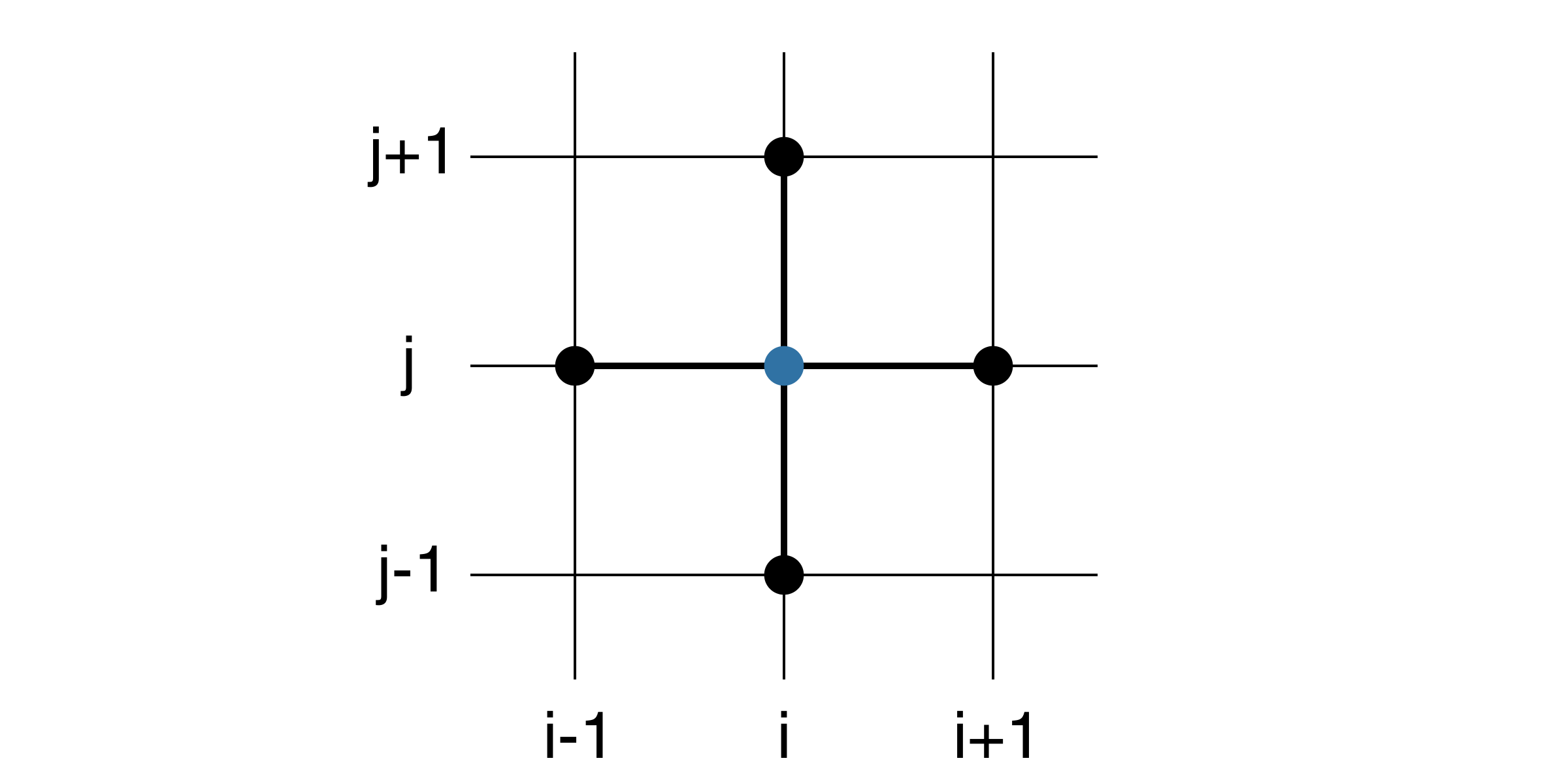
The resulting numerical stencil is shown in Figure 75.

It is easy to note that in (6.15), the value for the central point is the mean of the values of surrounding points. Equation (6.15) is very well-known and is usually called the 5-point formula (used in Chapter (6 Elliptic partial differential equations) ).

A problem arises at boundaries when using central differences. At those locations the stencil might fall outside of the computational domain and special strategies must be adopted. For example, one can replace central differences with backward or forward differences, depending on the case. Here we report some of these formulas with 2nd order accuracy.

Forward difference: $$ \begin{equation} \tag{6.16} \frac{\partial u}{\partial x}\bigg|_ {i,j} = \frac{-3u_{i,j}+4u_{i+1,j}-u_{i+2,j}}{2\Delta x} \end{equation} $$

Backward difference: $$ \begin{equation} \tag{6.17} \frac{\partial u}{\partial x}\bigg|_ {i,j} = \frac{3u_{i,j}-4u_{i-1,j}+u_{i-2,j}}{2\Delta x} \end{equation} $$

The formulas for forward , backward and central differences given in the chapter 2 Initial value problems for Ordinary Differential Equations can be used now if equipped with two indexes. A rich collection of difference formulas can be found in Anderson [11]. Detailed derivations are given in Hirsch [12].

6.3 Direct numerical solution

In situations where the elliptic PDE corresponds to the stationary solution of a parabolic problem (6.5), one may naturally solve the parabolic equation until stationary conditions occurs. Normally, this will be time consuming task and one may encounter limitations to ensure a stable solution. By disregarding such a timestepping approach one does not have to worry about stability. Apart from seeking a fast solution, we are also looking for schemes with efficient storage management a reasonable programming effort.

Let us start by discretizing the stationary heat equation in a rectangular plated with dimension as given in Figure 76: $$ \begin{equation} \frac{\partial^2 T}{\partial x^2} + \frac{\partial^2 T}{\partial y^2}=0 \tag{6.18} \end{equation} $$

We adopt the following notation: $$ \begin{align*} x_i&=x_0+i\cdot h,\ i=0,1,2,\dots\\ y_j&=y_0+j\cdot h,\ j=0,1,2,\dots \end{align*} $$ For convenience we assume \( \Delta x = \Delta y = h \). The ordering of the unknown temperatures is illustrated in (77).

By approximation the second order differentials in (6.18) by central differences we get the following numerical stencil: $$ \begin{equation} T_{i+1,j}+T_{i-1,j}+T_{i,j+1}+T_{i,j-1}-4 T_{i,j}=0 \tag{6.19} \end{equation} $$

which states that the temperature \( T_{i,j} \) in at the location \( (i,j) \) depends on the values of its neighbors to the left, right, up and down. Frequently, the neighbors are denoted in compass notation, i.e. \( \text{west}=i-1 \), \( \text{east}=i+1 \), \( \text{south}=j-1 \), and \( \text{north}=j+1 \). By referring to the compass directions with their first letters, and equivalent representation of the stencil in (6.19) reads: $$ \begin{equation} T_{e}+T_{w}+T_{n}+T_{s}-4 T_{m}=0 \tag{6.20} \end{equation} $$

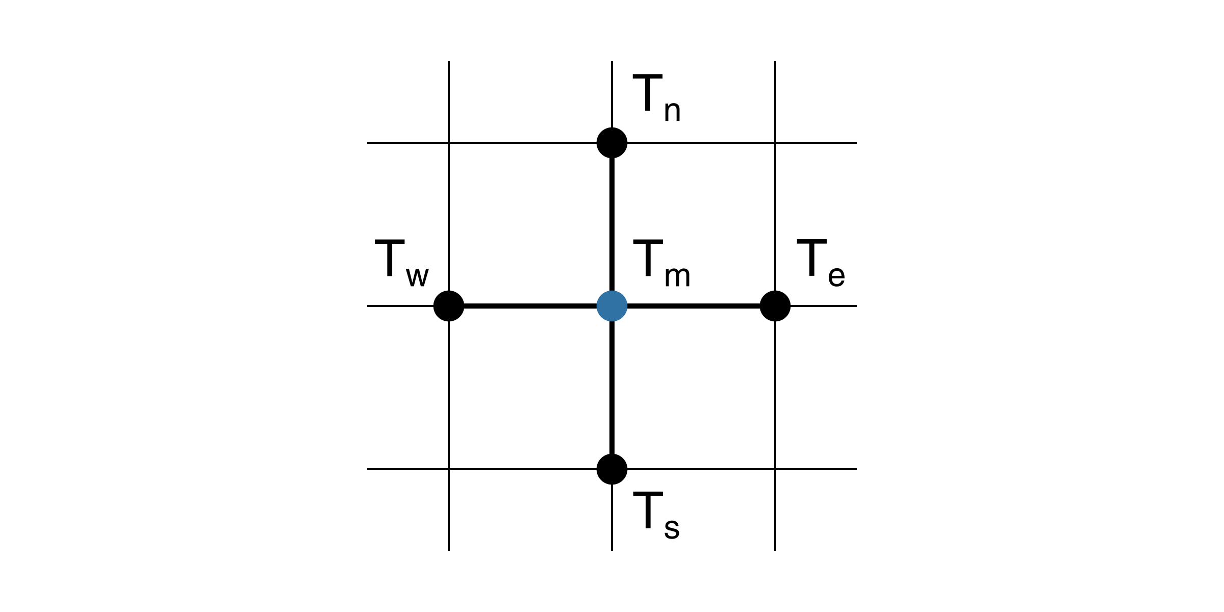
The smoothing nature of elliptic problems may be seen even more clearly by isolating the \( T_{i,j} \) in (6.20) on the left hand side: $$ \begin{equation} T_{m}= \frac{T_{e}+T_{w}+T_{n}+T_{s}}{4} \tag{6.21} \end{equation} $$ showing that the temperature \( T_{m} \) in each point is the average temperature of the neighbors (to the east, west, north, and south).

The temperature is prescribed at the boundaries (i.e. Dirichlet boundary conditions) and are given by: $$ \begin{align} T&=0.0 \quad \textrm{at} \quad y=0 \nonumber \\ T&=0.0 \quad \textrm{at} \quad x=0 \quad \textrm{ and }\quad x=1 \quad \textrm{ for } \quad 0 \leq y < 1.5 \tag{6.22}\\ T&=100.0 \quad \textrm{at} \quad y=1.5 \nonumber \end{align} $$

Our mission is now to find the temperature distribution over the plate by using (6.19) and (6.22) with \( \Delta x = \Delta y = 0.25 \). In each discretized point in (77) the temperatures need to satisfy (6.19), meaning that we have to satisfy as many equations as we have unknown temperatures. As the temperatures in each point depends on their neighbors, we end up with a system of algebraic equations. To set up the system of equations we traverse our unknowns one by one in a systematic manner and make use of use of (6.19) and (6.22) in each. All unknown temperatures close to any of the boundaries (left, right, top, bottom) in Figure 76 will be influenced by the prescribed and known temperatures the wall via the 5-point stencil (6.19). Prescribed values do not have to be calculated an can therefore be moved to the right hand side of the equation, and by doing so we modify the numerical stencil in that specific discretized point. In fact, inspection of Figure 76, reveals that only three unknown temperatures are not explicitly influenced by the presences of the wall (\( T_{2,2} \), \( T_{2,3} \), and \( T_{2,3} \)). The four temperatures in the corners (\( T_{1,1} \),$T_{1,5}$, \( T_{3,1} \), and \( T_{3,5} \)) have two prescribed values to be accounted for on the right hand side of their specific version of the generic numerical stencil (6.19). All other unknown temperatures close to the wall have only one prescribed value to be accounted for in their specific numerical stencil.

By starting at the lower left corner and traversing in the y-direction first, and subsequently in the x-direction we get the following system of equations: $$ \begin{align} -4\cdot T_{11}+T_{12}+T_{21}&=0 \nonumber\\ T_{11}-4\cdot T_{12}+T_{13}+T_{22} &=0 \nonumber\\ T_{12}-4\cdot T_{13}+T_{14}+T_{23}&=0 \nonumber\\ T_{13}-4\cdot T_{14}+T_{15}+T_{24} &=0 \nonumber\\ T_{14}-4\cdot T_{15}+T_{25}&=-100 \nonumber\\ T_{11}-4\cdot T_{21}+T_{22}+T_{31}&=0 \nonumber\\ T_{12}+T_{21}-4\cdot T_{22}+T_{23}+T_{32}&=0 \nonumber \\ T_{13}+T_{22}-4\cdot T_{23}+T_{24}+T_{33}&=0 \tag{6.23} \\ T_{14}+T_{23}-4\cdot T_{24}+T_{25}+T_{34}&=0 \nonumber \\ T_{15}+T_{24}-4\cdot T_{25}+T_{35}&=100 \nonumber \\ T_{21}-4\cdot T_{31}+T_{32}&=0,\nonumber \\ T_{22}+T_{31}-4\cdot T_{32}+T_{33}&=0 \nonumber \\ T_{23}+T_{32}-4\cdot T_{33}+T_{34}&=0 \nonumber \\ T_{24}+T_{33}-4\cdot T_{34}+T_{35}&=0 \nonumber \\ T_{25}+T_{34}-4\cdot T_{35}&=-100 \nonumber \end{align} $$

The equations in (6.23) represent a linear, algebraic system of equations with \( 5\times3=15 \) unknowns, which has the more convenient and condensed symbolic representation: $$ \begin{equation} \mathbf{A\cdot T=b} \tag{6.24} \end{equation} $$

where \( \mathbf{A} \) denotes the coefficient matrix, \( \mathbf{T} \) holds the unknown temperatures, and \( \mathbf{b} \) the prescribed boundary temperatures. Notice that the structure of the coefficient matrix \( \mathbf{A} \) is completely dictated by the way the unknown temperatures are ordered. The non-zero elements in the coefficient matrix are markers for which unknown temperatures are coupled with each other. Below we will show an example where we order the temperatures in y-direction first and then x-direction. In this case, the components of the coefficient matrix \( \mathbf{A} \) and the temperature vector \( \mathbf{T} \) are given by: $$ \begin{equation} \left(\begin{array}{ccccccccccccccc} -4& 1 & 0 & 0 & 0 & 1 & 0 & 0 & 0 & 0 & 0 & 0 & 0 & 0 &0 \\ 1& -4 & 1 & 0 & 0 & 0 & 1 & 0 & 0 & 0 & 0 & 0 & 0 & 0 &0 \\ 0& 1 & -4 & 1 & 0 & 0 & 0 & 1 & 0 & 0 & 0 & 0 & 0 & 0 &0 \\ 0& 0 & 1 & -4 & 1 & 0 & 0 & 0 & 1 & 0 & 0 & 0 & 0 & 0 &0 \\ 0& 0 & 0 & 1 & -4 & 0 & 0 & 0 & 0 & 1 & 0 & 0 & 0 & 0 &0 \\ 1& 0 & 0 & 0 & 0 & -4 & 1 & 0 & 0 & 0 & 1 & 0 & 0 & 0 &0 \\ 0& 1 & 0 & 0 & 0 & 1 & -4 & 1 & 0 & 0 & 0 & 1 & 0 & 0 &0 \\ 0& 0 & 1 & 0 & 0 & 0 & 1 & -4 & 1 & 0 & 0 & 0 & 1 & 0 &0 \\ 0& 0 & 0 & 1 & 0 & 0 & 0 & 1 & -4 & 1 & 0 & 0 & 0 & 1 &0 \\ 0& 0 & 0 & 0 & 1 & 0 & 0 & 0 & 1 & -4 & 0 & 0 & 0 & 0 &1 \\ 0& 0 & 0 & 0 & 0 & 1 & 0 & 0 & 0 & 0 & -4 & 1 & 0 & 0 &0 \\ 0& 0 & 0 & 0 & 0 & 0 & 1 & 0 & 0 & 0 & 1 & -4 & 1 & 0 &0 \\ 0& 0 & 0 & 0 & 0 & 0 & 0 & 1 & 0 & 0 & 0 & 1 & -4 & 1 &0 \\ 0& 0 & 0 & 0 & 0 & 0 & 0 & 0 & 1 & 0 & 0 & 0 & 1 & -4 &1 \\ 0& 0 & 0 & 0 & 0 & 0 & 0 & 0 & 0 & 1 & 0 & 0 & 0 & 1 &-4 \end{array}\right) \cdot \left(\begin{array}{c} T_{11}\\ T_{12}\\ T_{13}\\ T_{14}\\ T_{15}\\ T_{21}\\ T_{22}\\ T_{23}\\ T_{24}\\ T_{25}\\ T_{31}\\ T_{32}\\ T_{33}\\ T_{34}\\ T_{35} \end{array}\right) = \left(\begin{array}{c} 0\\ 0\\ 0\\ 0\\ -100\\ 0\\ 0\\ 0\\ 0\\ -100\\ 0\\ 0\\ 0\\ 0\\ -100 \end{array}\right) \tag{6.25} \end{equation} $$

The analytical solution of (6.18) and (6.22) may be found to be: $$ \begin{align} &T(x,y)=100\cdot \sum^\infty_{n=1}A_n\sinh(\lambda_ny)\cdot \sin(\lambda_nx) \tag{6.26}\\ &\textrm{where } \lambda_n = \pi\cdot n \textrm{ and } A_n=\frac{4}{\lambda_n\sinh(\frac{3}{2}\lambda_n)} \nonumber \end{align} $$

The analytical solution of the temperature field \( T(x,y) \) in (6.26) may be proven to be symmetric around \( x = 0.5 \) (see Exercise 9: Symmetric solution).

We immediately realize that it may be inefficient to solve (6.25) as it is, due to the presence of all the zero-elements. The coefficient matrix \( \mathbf{A} \) has \( 15\times 15=225 \) elements, out of which on 59 are non-zero. Further, a symmetric, band structure of \( \mathbf{A} \) is evident from (6.25). Clearly, these properties may be exploited to construct an efficient scheme which does not need to store all non-zero elements of \( \mathbf{A} \).

SciPy offers a sparse matrix package scipy.sparse, which has been used previously (see the section 4.4.1.1 Numerical solution).

# src-ch7/laplace_Diriclhet1.py
import numpy as np
import scipy 
import scipy.linalg
import scipy.sparse
import scipy.sparse.linalg
import matplotlib; matplotlib.use('Qt4Agg')
import matplotlib.pylab as plt
import time
from math import sinh

#import matplotlib.pyplot as plt
# Change some default values to make plots more readable on the screen
LNWDT=2; FNT=15
plt.rcParams['lines.linewidth'] = LNWDT; plt.rcParams['font.size'] = FNT

# Set simulation parameters
n = 15
d = np.ones(n) # diagonals
b = np.zeros(n) #RHS
d0 = d*-4
d1 = d[0:-1]
d5 = d[0:10]

A = scipy.sparse.diags([d0, d1, d1, d5, d5], [0, 1, -1, 5, -5], format='csc')

#alternatively (scalar broadcasting version:)
#A = scipy.sparse.diags([1, 1, -4, 1, 1], [-5, -1, 0, 1, 5], shape=(15, 15)).toarray()

# update A matrix
A[4, 5], A[5, 4], A[10, 9], A[9, 10] = 0, 0, 0, 0
# update RHS:
b[4], b[9], b[14] = -100, -100, -100
#print A.toarray()


tic=time.time()
theta = scipy.sparse.linalg.spsolve(A,b) #theta=sc.linalg.solve_triangular(A,d)
toc=time.time()
print('sparse solver time:',toc-tic)

 
tic=time.time()
theta2=scipy.linalg.solve(A.toarray(),b)
toc=time.time()
print('linalg solver time:',toc-tic)

# surfaceplot:
x = np.linspace(0, 1, 5)
y = np.linspace(0, 1.5, 7)

X, Y = np.meshgrid(x, y)

T = np.zeros_like(X)

T[-1,:] = 100

for n in range(1,6):
    T[n,1] = theta[n-1]
    T[n,2] = theta[n+5-1]
    T[n,3] = theta[n+10-1]
    
from mpl_toolkits.mplot3d import Axes3D
from matplotlib import cm
from matplotlib.ticker import LinearLocator, FormatStrFormatter
import numpy as np

fig = plt.figure()
ax = fig.gca(projection='3d')
surf = ax.plot_surface(X, Y, T, rstride=1, cstride=1, cmap=cm.coolwarm,
                       linewidth=0, antialiased=False)
ax.set_zlim(0, 110)

ax.zaxis.set_major_locator(LinearLocator(10))
ax.zaxis.set_major_formatter(FormatStrFormatter('%.02f'))
ax.set_xlabel('x')
ax.set_ylabel('y')
ax.set_zlabel('T [$^o$C]')
ax.set_xticks(x)
ax.set_yticks(y)

fig.colorbar(surf, shrink=0.5, aspect=5)
plt.show()

A somewhat more complicated solution of (6.18) may be found by specifying the different temperatures on all four boundaries. However, the code structure follows the same way of reasoning as for the previous example:

# src-ch7/laplace_Diriclhet2.py
import numpy as np
import scipy 
import scipy.linalg
import scipy.sparse
import scipy.sparse.linalg
import matplotlib; matplotlib.use('Qt4Agg')
import matplotlib.pylab as plt
import time
from math import sinh

#import matplotlib.pyplot as plt

# Change some default values to make plots more readable on the screen
LNWDT=2; FNT=15
plt.rcParams['lines.linewidth'] = LNWDT; plt.rcParams['font.size'] = FNT

# Set temperature at the top
Ttop=100
Tbottom=10
Tleft=10.0
Tright=10.0

xmax=1.0
ymax=1.5
 
# Set simulation parameters
#need hx=(1/nx)=hy=(1.5/ny)
Nx = 20
h=xmax/Nx
Ny = int(ymax/h)

nx = Nx-1
ny = Ny-1
n = (nx)*(ny) #number of unknowns
print(n, nx, ny)

d = np.ones(n) # diagonals
b = np.zeros(n) #RHS
d0 = d*-4
d1 = d[0:-1]
d5 = d[0:-ny]

A = scipy.sparse.diags([d0, d1, d1, d5, d5], [0, 1, -1, ny, -ny], format='csc')

#alternatively (scalar broadcasting version:)
#A = scipy.sparse.diags([1, 1, -4, 1, 1], [-5, -1, 0, 1, 5], shape=(15, 15)).toarray()

# set elements to zero in A matrix where BC are imposed
for k in range(1,nx):
    j = k*(ny)
    i = j - 1
    A[i, j], A[j, i] = 0, 0
    b[i] = -Ttop

b[-ny:]+=-Tright  #set the last ny elements to -Tright       
b[-1]+=-Ttop      #set the last element to -Ttop
b[0:ny-1]+=-Tleft #set the first ny elements to -Tleft 
b[0::ny]+=-Tbottom #set every ny-th element to -Tbottom

tic=time.time()
theta = scipy.sparse.linalg.spsolve(A,b) #theta=sc.linalg.solve_triangular(A,d)
toc=time.time()
print('sparse solver time:',toc-tic)
 
tic=time.time()
theta2=scipy.linalg.solve(A.toarray(),b)
toc=time.time()
print('linalg solver time:',toc-tic)

# surfaceplot:
x = np.linspace(0, xmax, Nx + 1)
y = np.linspace(0, ymax, Ny + 1)

X, Y = np.meshgrid(x, y)

T = np.zeros_like(X)


# set the imposed boudary values
T[-1,:] = Ttop
T[0,:] = Tbottom
T[:,0] = Tleft
T[:,-1] = Tright


for j in range(1,ny+1):
    for i in range(1, nx + 1):
        T[j, i] = theta[j + (i-1)*ny - 1]

    
from mpl_toolkits.mplot3d import Axes3D
from matplotlib import cm
from matplotlib.ticker import LinearLocator, FormatStrFormatter

fig = plt.figure()
ax = fig.gca(projection='3d')
surf = ax.plot_surface(X, Y, T, rstride=1, cstride=1, cmap=cm.coolwarm,
                       linewidth=0, antialiased=False)
ax.set_zlim(0, Ttop+10)
ax.set_xlabel('x')
ax.set_ylabel('y')
ax.set_zlabel('T [$^o$C]')


nx=4
xticks=np.linspace(0.0,xmax,nx+1)
ax.set_xticks(xticks)

ny=8
yticks=np.linspace(0.0,ymax,ny+1)
ax.set_yticks(yticks)

nTicks=5
dT=int(Ttop/nTicks)
Tticklist=list(range(0,Ttop+1,dT))
ax.set_zticks(Tticklist)

#fig.colorbar(surf, shrink=0.5, aspect=5)
plt.show()

Numerical values are listed below with analytical values from (6.26) enclosed in parentheses. $$ \begin{align*} &T_{11}=T_{31}=1.578\ (1.406),\ T_{12}=T_{32}=4.092\ (3.725)\\ &T_{13}=T_{33}=9.057\ (8.483),\ T_{14}=T_{34}=19.620\ (18.945)\\ &T_{15}=T_{35}=43.193\ (43.483),\ T_{21}=2.222\ (1.987),\ T_{22}=5.731\ (5.261)\\ &T_{23}=12.518\ (11.924),\ T_{24}=26.228\ (26.049),\ T_{25}=53.154\ (54.449) \end{align*} $$

The structure of the coefficient matrix will not necessarily be so regular in all cases, e.g. more complicated operators than the Laplace-operator or even more so for non-linear problems. Even though the matrix will predominantly be sparse also for these problems, the requirements for fast solutions and efficient storage will be harder to obtain for the problems. For such problems iterative methods are appealing, as they often are relatively simple to program and offer effective memory management. However, they are often hampered by convergence challenges. We will look into iterative methods in a later section.

• «
• 1
• ...
• 48
• 49
• 50
• 51
• 52
• 53
• 54
• 55
• 56
• 57
• 58
• 59
• 60
• 61
• 62
• 63
• 64
• 65
• ...
• 79
• »