Example 4.3: The Effect of Nonlinear Diffusion
This example shows the effect of nonlinear diffusion for the equation
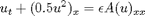
with Neumann boundary condition on an interval.
Initial setup
xmin=-1.5; xmax=1.5; T=1.0;
N = 255;
h = (xmax-xmin)/N; x=xmin+(0:N)*h;
u0 = -(abs(x)<=1.0).*sin(pi*x);
nstep=64;
Diffusion functions
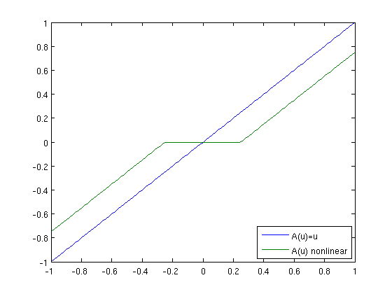
We will use two different diffusion functions: a linear function A(u)=u and a nonlinear function given by

The latter function is constant on the interval [-1/4,1/4], and here the parabolic equation degenerates and becomes hyperbolic.
u = linspace(-1,1,101);
plot(u,iden(u), u, Anonlin(u)), legend('A(u)=u','A(u) nonlinear',4)
Linear diffusion
For the linear diffusion, we compute the solution for two different choices of the parameter \epsilon that determines the balance between convective and diffusive forces
epsilon=0.1;
u=diffBurg('iden',u0,epsilon,h,1,nstep,'neumann');
u1=u(:,nstep+1);
epsilon=0.01;
u=diffBurg('iden',u0,epsilon,h,1,nstep,'neumann');
u2=u(:,nstep+1);
Nonlinear diffusion
Similarly, compute the solution for two different sizes of the diffusion parameter \epsilon
epsilon=0.5;
u=diffBurg('Anonlin',u0,epsilon,h,1,nstep,'neumann');
u3=u(:,nstep+1);
epsilon=0.05;
u=diffBurg('Anonlin',u0,epsilon,h,1,nstep,'neumann');
u4=u(:,nstep+1);
Discussion
subplot(1,2,1);
plot(x,u1,x,u2,'--'); xlabel('\it x'); ylabel('\it u');
legend('\epsilon=0.1','\epsilon=0.01'); axis([xmin xmax -0.75 0.75]);
title('Linear diffusion');
subplot(1,2,2);
plot(x,u3,x,u4,'--'); xlabel('\it x'); ylabel('\it u');
legend('\epsilon=0.5','\epsilon=0.05'); axis([xmin xmax -0.75 0.75]);
title('Nonlinear diffusion');
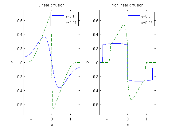
With the linear diffusion function, the solution is uniformly parabolic, and although the solution develops a sharp gradient in the vincinity of the origin for \epsilon=0.01, it remains smooth. For the nonlinear diffusion function, on the other hand, the solution degenerates with a hyperbolic region for u in [-1/4,1/4]. In the hyperbolic region, there are no viscous forces and the solution has developed a stationary shock at the origin. Notice also the nonsmooth transitions between the hyperbolic and the parabolic regions for \epsilon=0.05.