Example 2.7: Hyperbolic Conservation Laws in 2D

In this example we will solve the 2D scalar conservation law

$u_t + f(u)_x + g(u)_y = 0, \qquad u(x,y,0) = u_0(x,y)$

by dimensional splitting. To this end, we use two substeps,

$S_x(t): \quad v_t + f(v)_x = 0, \qquad v(x,0)=v_0(x)$

$S_y(t): \quad w_t + g(w)_y = 0, \qquad w(y,0)=w_0(y)$

and construct the approximate solution from the formula

$u(x,t)\approx [S_y(\Delta t)\circ S_x(\Delta t) ]^n u_0(x)$

The 1-D hyperbolic steps will be solved using the Lax-Friedrichs scheme

Initial setup

N = 256;
h = 2*pi/N;
x =-pi+(0:N)*h;  x=0.5*(x(1:end-1)+x(2:end));
y = x;
[X,Y] = ndgrid(x,y);
u0 = exp( -4*sin(X/2).^2 - 4*sin(Y/2).^2 );
h=path; path(h,'../Example2_5');

Flux functions

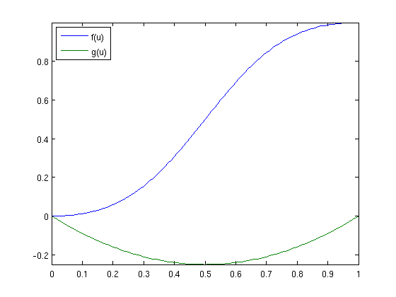
As a concrete example, we choose the Buckley-Leverett flux in the x-direction and a convex flux in the y-direction

$f(u) = u^2 / (u^2 + (1-u)^2), \qquad g(u) = u(1-u)$

This system can be seen as a simplified model of two-phase flow in a periodic porous medium under the influence of convective and gravity forces (convective in the x-direction and gravity in the y-direction). The two fluxes are shown in the plot below

u = linspace(0,1,101);
plot(u, fflux(u), u, gflux(u)), axis tight, legend('f(u)','g(u)',2)

Evolution of the solution

T = 1.5;
nsplit = 50;
u = dimsplit('fflux','gflux', u0, x, y, T, nsplit);
I = 1:10:nsplit+1;
t = linspace(0,T,nsplit+1);
c = linspace(0,1,11);
for i=1:6
   subplot(2,3,i),
   contourf(x,y,u(:,:,I(i))',c), caxis([0 1]) %, colorbar('horiz')
   %surf(x,y,u(:,:,I(i))'), shading interp, view(3)
   title(['Time: t=' num2str(t(I(i)))]);
end

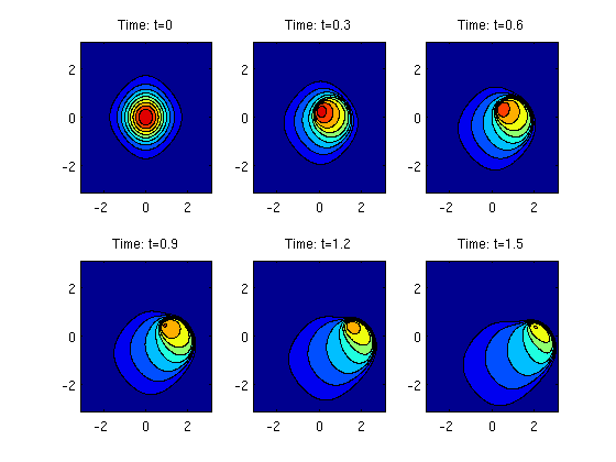
To understand the evolution of the initial blob, we discuss the movement in the two spatial directions separately. In the x-direction, the nonconvex Buckley-Leverett flux will turn the right-hand side of the symmetric blob into a leading shock, followed by a rarefaction. Likewise, the left-hand side of the blob turns into a shock followed by a rarefaction wave. In the y-direction, the convex flux gives a shock along the upper part of the blob and a rarefaction wave along the lower part.

Compare different time steps

Having established the dynamics of the problem, we can investigate the performance of our numerical method for different choices of the splitting step. To this end, we increase time interval to [0,8].

T = 8;
c = linspace(0,.25,11);
for n=1:4,
	nsplit=4*2.^(n-1);
	u=dimsplit('fflux','gflux',u0,x,y,T,nsplit);
	subplot(2,2,n)
	contourf(x,y,u(:,:,nsplit+1)',c), caxis([0 .25]);
	xlabel('x'), ylabel('y','Rotation',0),  colorbar
	title([num2str(nsplit) ' steps']);
end;
path(h);

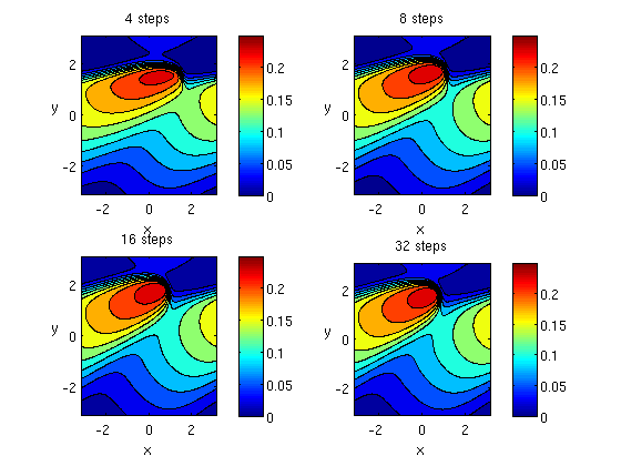
It is quite amazing how accurate one can capture the dynamics of this flow with only four splitting steps. Increasing the number of steps, improves small-scale features of the solution, but does not change the qualitative behavior of the approximate solution.