Example A.4: Burgers' Equation with Different Limiters
In this example we will study Burgers' equation
which is the archetypical example of a nonlinear equation, possessing a convex flux that may cause discontinuous shock waves to form even for smooth initial data. We assume Neumann boundary conditions and use a single shock as initial data to study the behavior of different limiters for a second-order high-resolution central scheme.
For this particular setup, we know the exact solution
xmin = 0; xmax=2;
T  = 3; NN = 512; hh=(xmax-xmin)/NN; xx=xmin+hh*(1:NN);
uexact = 1.0*(xx<(0.1+0.5*T));
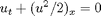
We consider four limiters (MinMod, vanLeer, MacCormack, and Superbee) and study the solution after 20 'passes' over the unit interval.
N   = 100; h=(xmax-xmin)/N; x=xmin+h*(1:N);
u0  = 1.0*(x<0.1);
CFL = 0.475;
limiter = {'minmod', 'vanleer', 'mc', 'superbee'};
name   = {'MinMod', 'vanLeer', 'MacCormack', 'Superbee'};
for i=1:4
   u=central('burgers',u0,T,h,1,'neumann',CFL,limiter{i});
   subplot(2,2,i);
   plot(xx,uexact,'-',x,u,'o','MarkerSize',4)
   axis([xmax-1 xmax -0.2 1.3]), title(name{i})
end
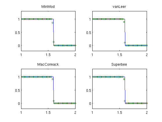
Because of the self-sharpening mechanisms in the propagating shock front, we only observe small differences in the resolution of the four limiters.