Dimensional Splitting: Front Tracking

In this example, we consider the 2D scalar conservation law

$u_t + (u^2/2)_x + (u^3/3)_y = 0, \qquad u(x,y,0)=u_0(x,y)$

which we solve using dimensional splitting. That is, we introduce two one-dimensional operators

$S_x(t): \quad v_t + (v^2/2)_x = 0, \qquad v(x,0)=v_0(x)$

$S_y(t): \quad w_t + (w^3/3)_y = 0, \qquad w(y,0)=w_0(y)$

and construct the approximate solution from the formula

$u(x,t)\approx [S_x(0.5\Delta t)\circ S_y(\Delta t)\circ S_x(0.5\Delta t) ]^n u_0(x)$

As a one-dimensional solver, we will use front tracking. This algorithm makes a piecewise constant approximation to the flux function and then solves the 1-D hyperbolic problem exactly, given piecewise constant initial data.

Disclaimer: The front-tracking code is built using arrays and is admittedly very slow, e.g., compared with the NT central-difference code. It is only meant to illustrate the concepts. For serious computing, one should use e.g., a C/C++ code built using pointers.

Initial setup

xmin=-1.0; xmax=1.0;
T = 2.0;
N = 50;
h = (xmax-xmin)/N;
x = xmin:h:xmax; y = 0.5*(x(1:end-1)+x(2:end));
[X,Y] = meshgrid(y,y);

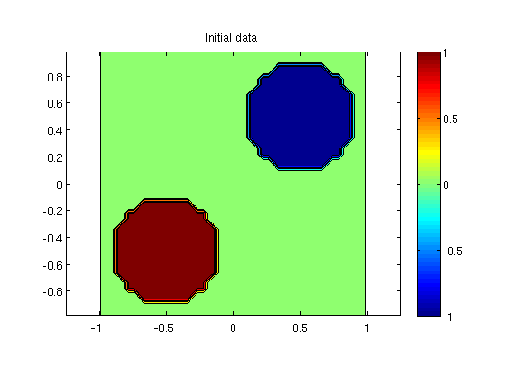
The initial function u0 is equal -1 inside a circle of radius 0.4 centered at (-1/2,-1/2), equal 1 inside a circle of radius 0.4 centered at (1/2,1/2), and zero otherwise. For later use, we define an anonymous function to do the computation of u0.

initData = (@(x,y) 1.0*((x+0.5).^2 + (y+0.5).^2 < 0.16) ...
   - 1.0*((x-0.5).^2 + (y-0.5).^2 < 0.16));
u0 = initData(X,Y);
contourf(X,Y,u0,-1:0.25:1); axis equal; colorbar, title('Initial data')

Number of time steps

In the first example, we fix the grid resolution and compare the approximate solutions generated with four different splitting steps (n=1, 4, 16, 64). Generally, it makes sense to match the resolution of the front-tracking algorithm with the grid resolution. The resolution of the front-tracking method is determined by segments in the piecewise linear approximation of the flux functions. Here, we simply scale these segments to be inversely proportional with sqrt(N).

for i=1:4,
   tic;
   u=DimSplit(u0,x,x,'burgerRsol','cubRsol',0.1/sqrt(N),4^(i-1), T,...
      'wbar','periodic',[xmin xmax],[xmin xmax]);
   t=toc; st=sprintf('%4.2f',t);

   subplot(2,2,i);
   contourf(y,y,u,30), axis equal image; colorbar
   title( sprintf('Grid: %dx%d  Steps: %d', N, N, 4^(i-1)));
   xlabel(['Time used: ', st,' sec.']);
   p=get(gca,'position'); p([3 4])=p([3 4])+0.03;
   set(gca,'position',p,'XTickLabel',[]);
end

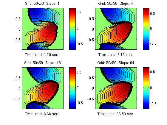
Looking at the plots, it is amazing to observe how well the operator splitting method resolves the dynamics of the problem using only one splitting step. The qualitative behavior of the red and blue "plumes" is captured almost correctly, even though the shape and position of the curved shock is not correct. Increasing the number of splitting steps to four (CFL number of 12.5) ensures that all qualitative features of the solution are captured correctly. For 64 time steps, the effective CFL number is less than one and the front-tracking method is equivalent to a standard Godunov method. By considering accuracy versus runtime, the optimal number of splitting steps is most likely somewhere between four and sixteen.

Increasing grid resolution

In the second example, we fix the CFL number to 20 and consider four different grid resolutions.

CFL=20;
for i=1:4,
   N= 32*(2^(i-1));
   h = (xmax-xmin)/N; delta=0.1/sqrt(N);
   x = xmin:h:xmax;
   y = 0.5*(x(1:end-1)+x(2:end));
   [X,Y] = meshgrid(y,y);
   u0=initData(X,Y);

   tic;
   Nstep=ceil(T/(CFL*h));
   u=DimSplit(u0,x,x,'burgerRsol','cubRsol',delta,Nstep,T,...
      'wbar','periodic',[xmin xmax],[xmin xmax]);
   t=toc; st=sprintf('%4.2f',t);

   subplot(2,2,i);
   pcolor(y,y,u), axis equal image; shading flat; colorbar
   title( sprintf('Grid: %dx%d, Steps: %d', N, N, Nstep));
   xlabel(['Time used: ', st,' sec.']);
   p=get(gca,'position'); p([3 4])=p([3 4])+0.03;
   set(gca,'position',p,'XTickLabel',[]);
end