Example 2.3: Linear Transport

Consider the linear hyperbolic equation

$u_t + au_x + bu_y = 0, \qquad u(x,y,0) = u_0(x,y).$

The equation describes the passive advection of a conserved quantity in a constant velocity field (a(x,y), b(x,y))

To solve this problem, we will use a Strang splitting, which is formally second order. The Strang splitting uses the two 1-D operators

$S_x(t):\quad v_t + a v_x = 0, \qquad v(x,0)=v_0(x)$

$S_y(t):\quad w_t + b w_y = 0, \qquad w(y,0)=w_0(y)$

and computes an approximate solution according to the formula

$u(x,y,t)\approx [S_x(\Delta t/2) \circ S_y(\Delta t)\circ S_x(\Delta t/2) ]^n u_0(x,y)$

The one-dimensional solution operators are approximated by the upwind method, which reads

$u_i^{n+1} = u_i^n - r \max(a_{i-1/2},0) (u_i - u_{i-1}) + r \min(a_{i+1/2},0) ( u_{i+1/2} - u_i)$

We study the properties of the solution operator using two numerical examples: constant transport along the diagonal and rotation around the origin.

Initial setup

We consider solution restricted to the domain [-5,5]x[-5,5]

N     = 128;
[xmin,xmax,ymin,ymax] = deal(-5, 5, -5, 5);
x = linspace(xmin,xmax,N+1);
y = linspace(ymin,ymax,N+1);
[X,Y] = meshgrid(x,y);

Constant transport along the diagonal

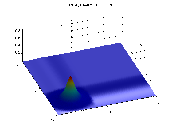
In the first example, we consider the transport of a Gaussian bell-shaped function in the direction (-1,-1).

U0    = exp(-2*sqrt((X-3).^2+(Y-3).^2));
a     = -ones(size(X));
b     = -ones(size(Y));
nstep = 3;
U     = transsplit(U0,a,b,x,y,6,nstep);

To investigate the accuracy of the solution, we plot the solution and compute the discrete L1-error. In the plot, we use the true solution (i.e., the initial solution transported to the correct location) to color our numerical approximation. As we can see from the plot, the colors appear to be symmetric and correctly placed on-top-of the approximate solution. This indicates that the operator splitting is correct for this particular problem and that the numerical errors we observe are only due to the upwind method used to approximate the 1-D solution operators.

surf(x, y, U(:,:,nstep+1), flipud(fliplr(U0))),
axis([xmin xmax ymin ymax min(min(U0)) max(max(U0))]);
shading interp; light, view(-20,60);
title(sprintf('%d steps, L1-error: %f', nstep, ...
      sum(sum(abs(U0-U(:,:,nstep+1))))/N^2));

Rotation about the origin

In the next example, we consider the rotation of a cylindric step function around the origin, as described by the equation

$u_t -y u_x + x u_y = 0, \qquad u(x,y,0)=1-H( 1 - (x-x_c)^2 - (y-y_c)^2)$

where H is the Heaviside function. This example is particularly well suited to study splitting errors that will appear immideately as a lack of symmetry in the solution. As in the previous example, we use the trick of using the true solution to color our approximate solution to reveal splitting errors.

a  = -Y; b = X;
r  = sqrt((X+1.8).^2+(Y+1.8).^2);
U0 = 1.0*(abs(r)<1.0);

for i=1:4
   nstep=2*2^i;
   U = transsplit(U0,a,b,x,y,2*pi,nstep);

   subplot(2,2,i), surf(x,y,U(:,:,nstep+1),U0),
   axis([xmin xmax ymin ymax min(min(U0)) max(max(U0))]);
   shading interp; light, view(-20,60);
   title(sprintf('%d steps, L1-error: %f', nstep, ...
      sum(sum(abs(U0-U(:,:,nstep+1))))/N^2));
   drawnow;
end

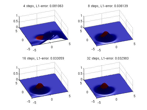
As we can see from the plots, the splitting method with four splitting steps fails to capture the correct solution. However, as the number of splitting steps increases, the approximate solution converges to the true solution and the dominating error comes from the finite-difference approximation of the 1-D solution operators.