Example A.1: Linear Advection in a Periodic Domain
The linear advection problem with periodic boundary conditions

is well suited for studying error mechanisms in numerical schemes for hyperbolic conservation laws. In particular, to study dissipative and oscillatory errors, we will use initial data consisting of a combination of a smooth, squared cosine wave and double step function.
We consider two first-order methods (Lax-Friedrichs and the upwind method) and two second-order methods (Lax-Wendroff and MacCormack)
T  = 10;
N  = 100; h=1/N; x=h*(1:N);
u0 = (abs(x-.25)<=0.15).*(cos(pi*(10/3)*(x-0.25))).^2 + ...
   1.0*(abs(x-0.75)<0.15);
xx  = linspace(0,1,1001);
uf  = (abs(xx-.25)<=0.15).*(cos(pi*(10/3)*(xx-0.25))).^2 + ...
   1.0*(abs(xx-0.75)<0.15);

method = {'LxF', 'upwind', 'LxW', 'McC'};
name   = {'Lax-Friedrichs', 'Upwind', 'Lax-Wendroff', 'MacCormack'};
for i=1:4
   u=finvol('linearfunc',u0,T,h,1,'periodic',method{i},.9);
   subplot(2,2,i);
   plot(xx,uf,'-',x,u,'o','MarkerSize',2); axis([0 1 -0.2 1.3]);
   title(name{i});
end
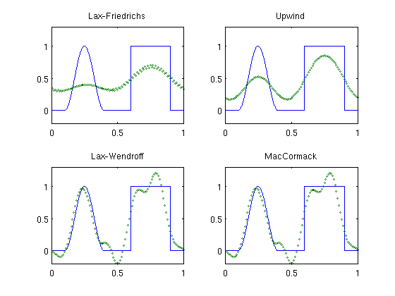
We see that the two first-order schemes smear both the smooth part and the discontinuous path of the advected profile and that the Lax-Friedrichs method is more diffusive than the upwind method. The second-order schemes, on the other hand, preserve the smooth profile quite accurately, but introduce spurious oscillations around the two discontinuities.