7.8 Wave travel and reflection

7.9 Networks 1D compliant vessels

The propagation of pressure and flow waves in the arterial system and how they influence stenotic regions, aneurysms and other vascular diseases, has been the subject of many studies [29] [30] [31] [32] [33] [34] [35] [28].

Recently there have also been a renewed interest for such 1D network models, as they both may provide valuable physiological insight in patient specific modalities (morphometric rendering of the arterial network) in addition to that they may provide better boundary conditions for 3D FSI models [36] [37] [38] [39] [40] [41].

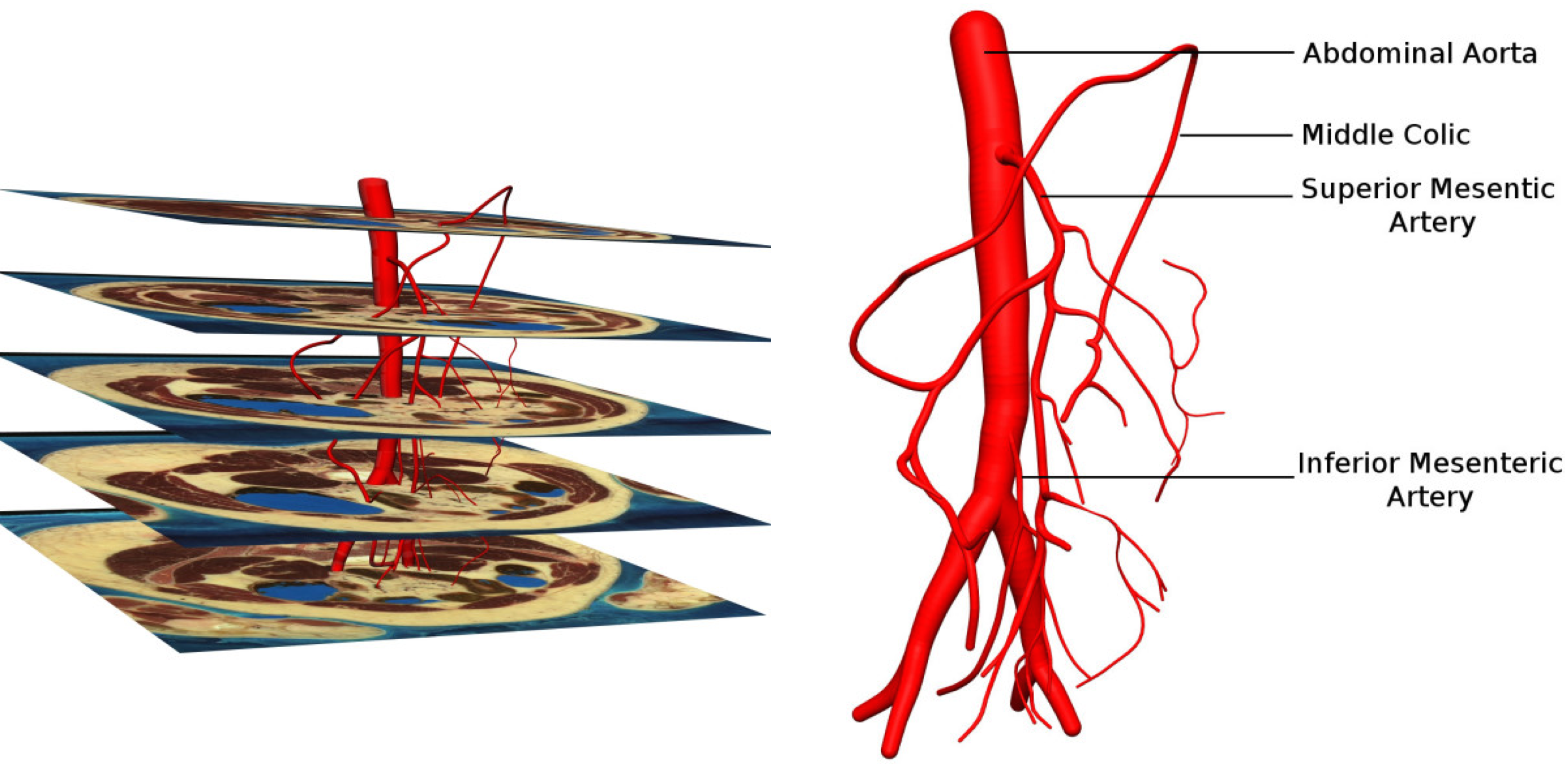
Network models have also been used for various segments of the arterial tree. To provide better understanding of the genesis of ischemia that develops in the gastrointestinal system, a model for the mesenteric arterial system have been developed to simulated realistic blood flow during normal conditions [42].

One of the early papers on this topic was on the blood flow in the human arm [43]. It used FEM to discretize the equations and a modified Windkessel model for the distal boundary conditions.

Figure 76: Anterior view of a subset of five images from the Visible Human dataset showing how the mesenteric arteries were created (from [42]).

A hybrid on-dimensional/Womersley model of pulsatile blood flow in the entire coronary arterial tree have also been developed recently[29].

Blood flow in the circle of Willis (CoW) has been modeled using the 1D equations of pressure and flow wave propagation in compliant vessels [44]. The model starts at the left ventricle and includes the largest arteries that supply the CoW. Based on published physiological data, it is able to capture the main features of pulse wave propagation along the aorta, at the brachiocephalic bifurcation and throughout the cerebral arteries.

\subsection{Numerical solution of the 1D equations for compliant vessels and boundary conditions}

When the governing 1D equations for compliant vessels (see e.g., equation (7.45) and (7.74)) are to be solved numerically, it is beneficial to recast them in the following generic form: $$ \begin{equation} \tag{7.128} \partd{\boldsymbol{u}}{t} + \boldsymbol{M} \partd{\boldsymbol{u}}{x} = 0 \end{equation} $$ In particular, the formulation equation (7.128) and what follows this section is important for the implementation of the boundary conditions. For the internal domain, any kind of numerical discretization may be employed.

By choosing the state vector as $ \boldsymbol{u} = [p,Q]^T $, the equations may be cast into the canonical given in equation (7.128) with: $$ \begin{equation} \tag{7.129} \boldsymbol{M} = \left [ \begin{array}{cc} \D 0 & \D \frac{1}{C} \\ \D \frac{A}{\rho} - (1+\delta) \, v^2 C & \D 2(1+\delta) \, v \end{array} \right ] \end{equation} $$ The off diagonal elements in $ \boldsymbol{M} $ represent a coupling in time and space between the components in the state vector, in this case the pressure $ p $ and the flow rate $ Q $.

In the following we will transform the equation system represented by equation (7.128), to a form where the rows of the equation system are independent. In order to do this we introduce the the diagonal eigenvalue-matrix of $ \boldsymbol{M} $ : $$ \begin{equation} \tag{7.130} \boldsymbol{\Lambda} = \left [ \begin{array}{cc} \lambda_1 & 0 \\ 0 & \lambda_2 \end{array} \right ] \end{equation} $$ the relation between $ \boldsymbol{M} $ and it's eigenvalues and corresponding eigenvectors may be written: $$ \begin{equation} \tag{7.131} \boldsymbol{M\,R} = \boldsymbol{R \, \Lambda} \end{equation} $$ The right eigenmatrix $ \boldsymbol{R} $ is composed of the right eigenvectors as columns. From basic linear algebra one may prove that the left eigenmatrix is $ \boldsymbol{L} $ related to the right eigenmatrix by $ \boldsymbol{L} = \boldsymbol{R}^{-1} $. The i-th row of $ \boldsymbol{L} $, denoted $ \boldsymbol{l}_i $, is the left eigenvector of $ \boldsymbol{M} $ corresponding to the i-th eigenvalue $ \lambda_i $. From equation (7.131) we see that $ \boldsymbol{M} = \boldsymbol{R \Lambda L} $ and thus by premultiplication of $ \boldsymbol{L} $ in equation (7.128), we obtain: $$ \begin{equation} \tag{7.132} \boldsymbol{L} \partd{\boldsymbol{u}}{t} + \boldsymbol{\Lambda L} \partd{\boldsymbol{u}}{x} = 0 \end{equation} $$ Further, we may introduce a change of variables such that $$ \begin{equation} \tag{7.133} \partd{\boldsymbol{\omega}}{\boldsymbol{u}} = \boldsymbol{L} \end{equation} $$ where $ \boldsymbol{\omega}=[\omega_1,\omega_2]^T $ is the vector of characteristic variables, also commonly denoted Riemann invariants, which in general satisfy: $$ \begin{equation} \tag{7.134} \boldsymbol{\omega} = \int_{\boldsymbol{u}_0}^{\boldsymbol{u}} \partd{\boldsymbol{\omega}}{\boldsymbol{u}} \, d\boldsymbol{u}= \int_{\boldsymbol{u}_0}^{\boldsymbol{u}} \boldsymbol{L} \, \, d\boldsymbol{u} \approx \boldsymbol{L}(\boldsymbol{u}_\epsilon) \, \Delta \boldsymbol{u}, \qquad \text{and} \quad \Delta \boldsymbol{u} = \boldsymbol{u}- \boldsymbol{u}_0 \end{equation} $$ The latter approximation follows from the mean value theorem (8.33) and is valid for some $ \boldsymbol{u}_0 \leq \boldsymbol{u}_\epsilon \leq \boldsymbol{u} $. In particular, the approximation is good if the change in the state variable vector from $ \boldsymbol{u}_0 $ to $ \boldsymbol{u} $ is small. This will typically be the case for an explicit numerical scheme where $ \boldsymbol{u}_0 $ refers to the state vector at the previous timestep and the timestep is small due to the CFL-limitation.

With this change of variables and use of the chain rule equation (7.132) transforms to a decoupled system of canonical wave equations: $$ \begin{equation} \tag{7.135} \partd{\boldsymbol{\omega}}{t} + \boldsymbol{\Lambda} \partd{\boldsymbol{\omega}}{x} = 0 \end{equation} $$ which on component form reads: $$ \begin{align} \partd{\omega_1}{t} + \lambda_1 \partd{\omega_1}{x} &= 0 \tag{7.136} \\ \partd{\omega_2}{t} + \lambda_2 \partd{\omega_2}{x} &= 0 \tag{7.137} \end{align} $$

For real eigenvalues $ \lambda_1 $ and $ \lambda_2 $, the Riemann invariants $ \omega_1 $ and $ \omega_2 $ are scalars which will propagate as waves, with wavespeeds $ \lambda_1 $ and $ \lambda_2 $, respectively. That is they have solutions: $$ \begin{align} \omega_1 & = \hat{\omega}_1 \, f(x-\lambda_1 t) \tag{7.138}\\ \omega_2 & = \hat{\omega}_2 \, g(x-\lambda_2 t) \tag{7.139} \end{align} $$ Note that when $ \lambda_1 $ and $ \lambda_2 $ have different signs, the waves will travel in opposite directions.

For our particular case in equation (7.129) on may find that the eigenvalues are: $$ \begin{align} \lambda_{1,2} &= (1+\delta) v \pm \sqrt{(1+\delta)^2 v^2 + c^2 - (1+\delta) v^2} \nonumber\\ & = \delta' v \pm c^* \tag{7.140} \end{align} $$ where we have introduced for simplicity: $$ \begin{equation} \tag{7.141} \delta' = (1+\delta), \qquad c^* = c \, \sqrt{1+\delta' (\delta ' -1) \mathcal{M}^2} \qquad \text{ and } \qquad\mathcal{M} =v/c \end{equation} $$ Here, $ c $ denote the invisicid pulse wave velocity as defined in equation (7.79). The $ \delta' $ is simply a modified correction factor, whereas $ c^* $ is the modified wave speed due to the velocity field, and $ \mathcal{M} $ is a Mach number. Note that a flat velocity profile corresponds to $ \delta = 0 $, and consequently $ \delta' =1 $ and $ c^*=c $. Normally, $ v \ll c^* $ and therefore we see from equation (7.140) that $ \lambda_1 > 0 $ and $ \lambda_2 < 0 $, and therefore $ \omega_1 $ will travel to the right (or in the positive coordinate direction) whereas $ \omega_2 $ will travel to the left (or in the negative coordinate direction) according to equation (7.136) and (7.137).

The corresponding left eigenmatrix may be taken as: $$ \begin{equation} \tag{7.142} \boldsymbol{L} = \left [ \begin{array}{cc} 1 & -1/\lambda_2 C \\ 1 & -1/\lambda_1 C \end{array} \right ] = \left [ \begin{array}{cc} 1 & Z_c^b\\ 1 & -Z_c^f \end{array} \right ] \approx \left [ \begin{array}{cc} 1 & Z_c\\ 1 & -Z_c \end{array} \right ] \end{equation} $$ where we have introduced the modified characteristic impedances for the forward and backward traveling waves as $ Z_c^f $ and $ Z_c^b $, respectively.

From equations (7.134) and (7.142) we get: $$ \begin{equation} \tag{7.143} \boldsymbol{\omega} = [\omega_1, \omega_2 ]^T = \boldsymbol{L}(\boldsymbol{u}_\epsilon) \, \Delta \boldsymbol{u} =[\Delta p + Z_c^b \Delta Q, \quad \Delta p - Z_c^f \Delta Q]^T \end{equation} $$ Note, that the $ Z_c^f = Z_c^f(p,Q) $ and $ Z_c^b = Z_c^b(p,Q) $, and are to be evalued in the given range $ \boldsymbol{u}_0 \leq \boldsymbol{u}_\epsilon \leq \boldsymbol{u} $. Normally, the value at the previous timestep may be used.

The Riemann invariants $ \boldsymbol{\omega} $ are conventionally found from the internal field and from the boundary conditions. Subsequently the updated values of the primary variables are found at the boundary by: $$ \begin{equation} \tag{7.144} \Delta \boldsymbol{u} = \boldsymbol{L}(\boldsymbol{u}_\epsilon)^{-1} \boldsymbol{\omega} = \boldsymbol{R}(\boldsymbol{u}_\epsilon) \boldsymbol{\omega} \end{equation} $$ where: $$ \begin{equation} \tag{7.145} \boldsymbol{R} = \frac{1 }{Z_c^f + Z_c^b} \left [ \begin{array}{cc} Z_c^f & Z_c^b\\ 1 & -1 \end{array} \right ] \approx \frac{1 }{2\, Z_c} \left [ \begin{array}{cc} Z_c & Z_c\\ 1 & -1 \end{array} \right ] \end{equation} $$

The increments in the primary variables may also be expressed by means of the Riemann invariants by rearrangements of the expressions in equation (7.143): $$ \begin{equation} \tag{7.146} \Delta Q = \frac{\omega_1 - \omega_2 }{Z_c^f + Z_c^b} , \qquad \Delta p = \frac{Z_c^f \omega_1 + Z_c^b \omega_2 }{Z_c^f + Z_c^b} \end{equation} $$ Note that for waves superimposed on a quiescent fluid fluid, i.e., for $ v=0 $ in equation (7.140), then $ \lambda_1 = -\lambda_2 $ and $ Z_c^f =Z_c^b = Z_c $, and consequently equation (7.146) simplifies to: $$ \begin{equation} \tag{7.147} \Delta Q = \frac{\omega_1 - \omega_2 }{2Z_c} , \qquad \Delta p = \frac{\omega_1 + \omega_2 }{2} \end{equation} $$ now we may define: $$ \begin{align} \tag{7.148} \Delta Q_f & = \frac{\omega_1}{Z_c^f + Z_c^b} , & \Delta Q_b & = \frac{-\omega_2}{Z_c^f + Z_c^b} \\ \Delta p_f & = \frac{Z_c^f\, \omega_1}{Z_c^f + Z_c^b} , & \Delta p_b & = \frac{Z_c^b \, \omega_2}{Z_c^f + Z_c^b} \tag{7.149} \end{align} $$ which by substitution into equation (7.146) yields: $$ \begin{align} \tag{7.150} \Delta Q & = \Delta Q_f + \Delta Q_b \\ \Delta p & = \Delta p_f + \Delta p_b \tag{7.151} \end{align} $$

7.9.0.1 Inlet boundary conditions

A prescribed flow at the inlet boundary may be imposed in such a way that the wave approaching this boundary from the interior field is also handled in a way which respects the physics or the differential equations for the problem. Clearly, as flow is imposed we know the value of $ Q_{in} $, the pressure, however, has to be computed and will be a function both of the flow at the inlet and of waves coming from the interior. The mathematical consequence of this outset is that two conditions need to be fulfilled, namely that the flow $ Q_{in} $ may be taken as a time varying function $ Q_{in}=Q(t) $, whereas the outgoing wave will be accounted for by imposing $ \boldsymbol{l_2 \cdot u_{in}} = \omega_2 $. Note we assume here that the inlet is taken at the left boundary, i.e., where the $ x $-coordinate is at minimum.

Now, to compute the resulting pressure from the imposed flow $ Q_{in} $ and the (potential) wave $ \omega_2 $ from the interior, we construct an equation system similar to equation (7.134). As we need to respect the physics from the interior we keep the second row of $ \boldsymbol{L} $, corresponding to the wave from the interior $ \omega_2 $, but modify the first row to ensure that the flow is imposed: $$ \begin{equation} \tag{7.152} \boldsymbol{L}_{in} \boldsymbol{u}_{in} = \boldsymbol{\omega}_{in} \end{equation} $$ where: $$ \begin{equation} \tag{7.153} \boldsymbol{L}_{in} = \left [ \begin{array}{cc} 0 & 1 \\ 1 & -Z_c^f \end{array} \right ] \quad \mathrm{and} \quad \boldsymbol{\omega}_{in} = \left [ \begin{array}{c} Q(t) \\ \omega_2 \end{array} \right ] \end{equation} $$ By inspecting equations (7.152) and (7.153), we see that the above mentioned conditions are satisfied. The inverse of $ \boldsymbol{L}_{in} $ may be computed as: $$ \begin{equation} \boldsymbol{L}_{in}^{-1} = \left [ \begin{array}{cc} Z_c^f & 1 \\ 1 & 0 \end{array} \right ] \tag{7.154} \end{equation} $$ and the resulting pressure $ p_{in} $ (and flow) from the imposed flow may be computed as:

Imposed flow $$ \begin{equation} \tag{7.155} \boldsymbol{u}_{in} = \left [ \begin{array}{c} p_{in} \\ Q_{in} \end{array} \right ] = \boldsymbol{L}_{in}^{-1} \cdot \boldsymbol{\omega}_{in} = \left [ \begin{array}{c} Z_c^f Q(t) + \omega_2 \\ Q(t) \end{array} \right ] \end{equation} $$

and we clearly see from equation (7.155), that the pressure has contributions from both the imposed flow and the wave from the interior $ \omega_2 $. Observe also that with no reflected wave present (i.e., $ \omega_2 = 0 $, pressure and flow are related with the characteristic impedane $ Z_c^f $, as expected.

A similar strategy may be taken for an imposed time varying pressure $ p_i = p(t) $: $$ \begin{equation} \boldsymbol{L}_{in} = \left [ \begin{array}{cc} 1 & 0 \\ 1 & -Z_c^f \end{array} \right ] \quad \mathrm{and} \quad \boldsymbol{L}_{in}^{-1} = \left [ \begin{array}{cc} 1 & 0 \\ -1/Z_c^f & 1/Z_c^f \end{array} \right ] \quad \mathrm{and} \quad \boldsymbol{\omega}_{in} = \left [ \begin{array}{c} p(t) \\ \omega_2 \end{array} \right ] \tag{7.156} \end{equation} $$ which yields the following equations for the inlet:

Imposed pressure $$ \begin{equation} \tag{7.157} \boldsymbol{u}_{in} = \left [ \begin{array}{c} p_{in} \\ Q_{in} \end{array} \right ] = \left [ \begin{array}{c} p(t) \\ \D \frac{\omega_2 - p(t)}{Z_c^f} \end{array} \right ] \end{equation} $$

We observe from equation (7.157) that the inlet flow $ Q_{in} $ has contributions both from the imposed pressure $ p(t) $ and from the interior wave $ \omega_2 $. In the absence of a reflected wave $ \omega_2 $, pressure and flow are related with the characteristic impdeance $ Z_c^f $ as expected for unidirectional waves.

7.9.0.2 Impose forward flow/pressure

Impose $ \Delta Q_f = Q_0 $. From equation (7.148) $ \omega_1 $ may be computed as: $$ \begin{equation} \tag{7.158} \omega_1 = (Z_c^f + Z_c^b) \Delta Q_f = (Z_c^f + Z_c^b) \Delta Q_0 \end{equation} $$ Extrapolation from interior field: $$ \begin{equation} \tag{7.159} \omega_2 = w_2(t^n, \lambda_2 \Delta t) \end{equation} $$ and compute values at the inlet by: $$ \begin{equation} \tag{7.160} \mathbf{\Delta u}_{in} = \mathbf{R} \boldsymbol{\omega} \end{equation} $$ The expressions in equation (7.158) may be simplified whenever $ v \ll c $ and concequently $ Z_c^f \approx Z_c^b =Z_c $ and thus: $$ \begin{equation} \tag{7.161} \omega_1 = 2 \, Z_c \Delta Q_0 \end{equation} $$ and the imposed primary variables then become:

Imposed forward flow $$ \begin{equation} \tag{7.162} \mathbf{\Delta u}_{in} = \left [ \begin{array}{c} p_{in} \\ Q_{in} \end{array} \right ] = \mathbf{R} \boldsymbol{\omega} = \left[ \begin {array}{c} Z_c \, Q_f+\omega_2/2 \\ Q_{f}-\omega_2/2 \,Z_c \end {array} \right] \end{equation} $$

7.9.0.3 Outlet boundary conditions

In the numerical scheme for the governing equations (7.45) and (7.74), a values for $ \omega_1 $ are $ \omega_2 $ are needed in order to prescribe the pressure/flow at the outlet in a way which repsects both the wave $ \omega_1 $ coming from the inside of the vessel and the wave entering the vessel $ \omega_2 $. This amounts to solving equation (7.144) at the boundary.

For the outlet (i.e., for $ x =L $) the outgoing Riemann invariant may be extrapolated from the interior field from the previous timestep. Whenever source terms are negligible in equation (7.136), the outgoing Riemann invariant at the outlet is constant along the characteristic curve $ dx/dt = \lambda_1 $, and thus we can approximate: $$ \begin{equation} \tag{7.163} \omega_1^{n+1} = \omega_1(t_n,L-\lambda_1^n \Delta t) \end{equation} $$

The question now is how one may obtain a value for $ \omega_2 $, which represents the incoming wave due to the two element Windkessel. Terminal vessels are often modeled with lumped models Windkessel model, which is represented by the differential equation (6.15). On incremental form the two element Windkessel mode has the corresponding differential equation: $$ \begin{align} \tag{7.164} \Delta Q & = C \partd{\Delta p}{t} + \frac{\Delta p}{R} \end{align} $$ Now, by substiution of equation (7.147), which expresses the primary variables $ p $, and $ Q $ by means of the Riemann invariants, into the differential equation (7.164) which models the physics of the exterior, a differential equation for $ \omega_2 $ is obtained: $$ \begin{equation} \tag{7.165} Z_c^b C \, \frac{d \omega_2}{dt} + \omega_2 \left (1 + \frac{Z_c^b}{R} \right ) = Z_c^f C \, \frac{d \omega_1}{dt} + \omega_1 \left (1 - \frac{Z_c^f}{R} \right ) \end{equation} $$ As the right hand side of equation (7.165) is known from previous values of $ \omega_1 $ and from the extrapolated current value given by equation (7.163), an updated value for $ \omega_2 $ may readily be obtained by an appropriate discretization of equation (7.165), e.g., backward Euler.

7.9.1 Lumped heart model: varying elastance model

The varying elastance model, is a phenemenological model of the left ventricular function, originally proposed [45] [46] $$ \begin{align} \tag{7.166} E(t) = \frac{p_v(t)}{V(t) - V_0} \end{align} $$

Modified version $$ \begin{align} \tag{7.167} E(t) = \frac{p_v(t)}{(V(t) - V_0) \, (1 + K Q_v(t))} \end{align} $$ with $ K $ as a resistance in the left ventricle. Normally, $ K $ is rather small, and therefore a first approximation is to assume it to be zero as in equation (7.166).

As $ V(t) $ is the instantaneous left ventricular volume, the flow rate $ Q_v(t) $ ejected by the left ventricle is given by $ Q_v(t) = - dV/dt $. From the varying elastance model in equation (7.166) we get: $$ \begin{align} \tag{7.168} Q_v(t) =- \frac{dV}{dt} = \frac{dE}{dt} \left (\frac{1}{E^2} \right ) \, p_v - \frac{1}{E} \, \frac{dp_v}{dt} \end{align} $$ from the representation we see that $ 1/E $ plays the role of a compliance and: $$ \begin{align} \tag{7.169} \frac{d}{dt} \left (\frac{1}{E} \right ) \end{align} $$ the role of a resistance [47].

The varying elastance model may be used as an inlet condition, subject to the assumption that $ Q=Q_v $ and $ p=p_v $ at the inlet. As we now are at the inlet, we may extraplate the outgoing Riemann invariant $ \omega_2 $ in the same manner as in equation (7.163): $$ \begin{equation} \tag{7.170} \omega_2^{n+1} = \omega_2(t_n,\lambda_2^n \Delta t) \end{equation} $$ Further, the differential equation for $ \omega_1 $ may be obtained by substitution of equation (7.146) into the differential equation (7.168) for the varying elastance model: $$ \begin{equation} \tag{7.171} \frac{Z_c^f}{E} \frac{d \omega_1}{dt} + \omega_1 \left (1- \frac{Z_c^f}{E^2} \frac{d E}{dt} \right ) = -\frac{Z_c^b}{E} \frac{d \omega_2}{dt} + \omega_2 \left (1+ \frac{Z_c^b}{E^2} \frac{d E}{dt} \right ) \end{equation} $$ Thus, an updated value at time level $ n+1 $ may be obtained for ($ \omega_1^{n+1} $) by e.g., a backward Euler dicretization of equation (7.171).

When, modelling the interaction of the heart and the cardiovacular system, one obviously have to account for the presence of the aortic valve and the fact that it is closed during diastole. The closure of the aortic valve is normally attributed to a negative pressure difference between the left ventricle and the aorta.

From equations (7.166) and (7.168) on may estimate an updated left ventricular pressure at the next time level: $$ \begin{equation} p_v^{n+1} = E(t) \left ( V_n - Q_n \Delta t - V_0 \right ) \tag{7.172} \end{equation} $$

The negative pressure difference criterion for valve closure will therefore be $ p_v < p^{n+1} $.

Whenever the valve is closed, there is no outflow from the heart which corresponds $ Q_v = 0 $ in equation (7.168). Note that despite a closed aortic valve, waves may still arrive from the periphery $ \omega_2 \neq 0 $, and such waves will be reflected at the closed valve. A complete reflection ($ \Gamma =1 $), is a first approximation which corresponds to $ \omega_1 = \omega_2 $).

The pressure criteria for valve closure together with the varying elastance model as inlet condition may therefore be summarized to: $$ \begin{equation} \tag{7.173} \omega_1 = \left \{ \begin{array}{c@{\text{ if }}c} (7.171) & p_v >p \\ \omega_2 & p_v \leq p \\ \end{array} \right . \end{equation} $$

7.9.2 Nonlinear wave separation

Expressions for nonlinear wave separation follow readily from equation (7.146) as $ \omega_1 $ is a forward propagating Riemann invariant and $ \omega_2 $ is a backward propagating Riemann invariant. The forward/backward propagating pressures and flows are found simply by setting $ \omega_2 = 0 $ and $ \omega_1 = 0 $, respectively, in equation (7.147): $$ \begin{align} \tag{7.174} \begin{aligned} \Delta Q_f &= \frac{\omega_1 }{Z_c^f + Z_c^b} , & \Delta Q_b &= \frac{- \omega_2 }{Z_c^f + Z_c^b} \\ \Delta p_f &= \frac{Z_c^f \omega_1 }{Z_c^f + Z_c^b}, & \Delta p_b & = \frac{Z_c^b \omega_2 }{Z_c^f + Z_c^b} \end{aligned} \tag{7.175} \end{align} $$ Naturally, for the more simpler case of a quiescent fluid fluid, the previously derived expressions for linear wave separation (see equation (7.126) and (7.127)) in the section 7.7 Wave separation) may be obtained from equation (7.147).