5 Fluid mechanics
5.1 Introduction
In a continuum mechanical setting, it is convenient to define a fluid based on the macro mechanical conditions which are the most prominent for a fluid or gass compared to a solid. Thus, we have chosen the
following definition:
For an anisotropic stress condition, one may always find planes with shear stress. A fluid will therefore deform contiuously while exposed to shear stress. Conversely, the fluid may be at rest for only isotropic stress states, and the constitutive equation for any fluid at rest (relative to a reference) may be expressed by the simple relation: $$ \begin{equation} \boldsymbol{T} = -p \, \boldsymbol{1}, \qquad p =p(\rho,\theta) \tag{5.1} \end{equation} $$ where \( p \) is the thermodynamical pressure which is a function of the density \( \rho \) and the temperature \( \theta \). % The expression for \( p \) on the right hand side of equation (5.1), is often referred to as an equation of state. A familiar example of the latter, is the equation of state for the ideal gas: $$ \begin{equation} p = R \rho \theta \tag{5.2} \end{equation} $$ where \( R \) is the gas constant for the gas, and \( \theta \) is the absolute temperature (in degrees Kelvin). % Note that, this equation of state is a model for an ideal gas, but may be used as a good approximation for many real gases, for example air.
Small fluid elements, or fluid particles, are in general exposed to large displacements and chaotic motions and it is impossible to follow the motion of the individual particles. A fixed position in space therefore normally used for the observation and mathematical representation of the velocity, pressure, and physical properties of fluids in motion.
Eulerian coordinates due to large displacements and chaotic motion of the individual fluid particles. The velocity vector \( \boldsymbol{v}(\boldsymbol{r},t) \) is the primary kinetic property
5.1.1 Fundamental concepts in fluid mechanics
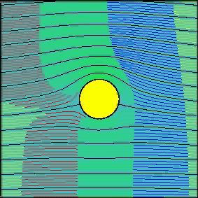
Stream lines Vector lines to the velocity field. Changes with time for non-steady flow \( \boldsymbol{v} = \boldsymbol{v}(\boldsymbol{r},t) \). Coincide with particle trajectories (path lines) for steady flow (\( \boldsymbol{v} = \boldsymbol{v}(\boldsymbol{r}) \)). Differential vector parallel with velocity vector implies: \( d\boldsymbol{r} \times \boldsymbol{v}(\boldsymbol{r},t) = 0 \).
Figure 35: Illustration of streamlines.
Path lines (particle trajectories): $$ \begin{equation} \dot{\boldsymbol{r}} = \boldsymbol{v}(\boldsymbol{r},t) \tag{5.3} \end{equation} $$ Vorticity field: $$ \begin{equation} \boldsymbol{c} = \nabla \times \boldsymbol{v} \tag{5.4} \end{equation} $$ Potential flow $$ \begin{equation} \boldsymbol{v} = \nabla \phi, \quad \phi=\phi(\boldsymbol{r},t) \quad \Leftarrow \nabla \times \boldsymbol{v} = 0 \tag{5.5} \end{equation} $$
The Reynolds number: Solutions to the governing equations may not be unique. Increasing velocities in a pipe will eventually produce chaotic unsteady flow. The Reynolds number predicts transition from laminar to turbulent flow. $$ \begin{equation} \Re = \frac{\rho \bar{v} d}{\mu}, \quad \bar{v} = \frac{Q}{A} \tag{5.6} \end{equation} $$
\( \rho \) density, \( \mu \) viscosity, \( d \) pipe diameter, \( Q \) flow rate \( [m^3/s] \), \( A \) pipe cross section
Turbulent flow when \( \Re > 2000 \).