3.4 Strain rates and rates of rotation

Eulerian coordinates and the current configuration $ K $ are commonly used to represent mathematically the motion and deformation of fluids, and sometimes solids with fluid like behavior.

The particles are in such a scenario denoted by the position vector $ \mathbf{r} $ in $ K $, rather than the original position $ \mathbf{r}_0 $ or $ X $. We then consider a particle $ P $ at location $ \mathbf{r} $ at time $ t $, with the velocity $ \mathbf{v}(\mathbf{r},t) $. During a short time increment $ dt $ the particle $ P $ is subjected to the displacement $ d\mathbf{u} = \mathbf{v} dt $, and associated small deformations given by the displacement tensor $ d\mathbf{H} $: $$ \begin{equation} \tag{3.75} dH_{ik} = \partd{v_i}{x_k} \,dt \equiv v_{i,k} \,dt \end{equation} $$ and accordingly a small strain tensor $ d\mathbf{E} $ (compare with Eq. (3.48) for small displacements) and a rotation tensor for small deformations $ d\tilde{\mathbf{R}} $: $$ \begin{equation} \tag{3.76} d\mathbf{E} = \frac{1}{2} \, \left ( d\mathbf{H} + d\mathbf{H}^T \right ), \qquad d\tilde{\mathbf{R}} = \frac{1}{2} \, \left ( d\mathbf{H} - d\mathbf{H}^T \right ) \end{equation} $$ As the velocity has entered the expressions in Eq. (3.75) and (3.76), three new tensors are defined as a consequence: the velocity gradient tensor $ \mathbf{L} $, the symmetric rate of deformation tensor $ \mathbf{D} $, and the antisymmetric rate of rotation tensor $ \mathbf{W} $: $$ \begin{align} \mathbf{L} & = \partd{\mathbf{v}}{\mathbf{r}} &\Leftrightarrow L_{ik} &= v_{i,k} \tag{3.77}\\ \tag{3.78} \mathbf{D} & = \frac{1}{2} \left ( \mathbf{L+L}^T \right ) &\Leftrightarrow D_{ik} &= \frac{1}{2} \left ( v_{i,k} + v_{k,i} \right ) \\ \mathbf{W} & = \frac{1}{2} \left ( \mathbf{L-L}^T \right ) &\Leftrightarrow W_{ik} &= \frac{1}{2} \left ( v_{i,k} - v_{k,i} \right ) \tag{3.79} \end{align} $$ The new definitions lead to: $$ \begin{align} d\mathbf{H} = \mathbf{L} dt, \qquad d\mathbf{E} = \mathbf{D} dt, \qquad d\tilde{\mathbf{R}} = \mathbf{W} dt, \qquad \dot{\mathbf{E}} = \mathbf{D}, \qquad \dot{\tilde{\mathbf{R}}} = \mathbf{W} \tag{3.80} \end{align} $$ Note that $ \dot{\mathbf{E}} $ is the material derivative of the small strain tensor from Eq. (3.48) for small deformations. In the general case relation between the material derivative om the general Green strain tensor $ \mathbf{E} $ as defined by Eq. (3.23) and the rate of deformation tensor $ \mathbf{D} $ is more complex.

The change of length of a material line per unit length and per unit time is denoted the rate of longitudinal strain \index{Rate of longitudinal strain} or for short rate of strain \index{rate of strain}. By arguing in the same manner as in the section 3.3.1 Small strains, it follows that the rate of strain in the direction $ \mathbf{n} $ is: $$ \begin{align} \dot{\epsilon} = \mathbf{n \cdot D \cdot n} \tag{3.81} \end{align} $$ In the coordinate directions $ \mathbf{e}_i $, we get the coordinate rates of strain : $$ \begin{align} \dot{\epsilon}_{ii} = D_{ii} = v_{i,i}, \qquad *no summation* \tag{3.82} \end{align} $$ and similarly the rate of shear strain \index{Rate of shear strain} or the shear rate with respect to two orthogonal lines $ \mathbf{n} $ and $ \mathbf{\bar{n}} $: $$ \begin{align} \dot{\gamma} = 2 \mathbf{\bar{n} \cdot D \cdot n} \tag{3.83} \end{align} $$ whereas the coordinate shear rate \index{Coordinate shear rate} for the direction $ \mathbf{e}_1 $ and $ \mathbf{e}_2 $ are given by: $$ \begin{align} \tag{3.84} \dot{\gamma}_{21} = 2 D_{21} = v_{2,1} + v_{1,2} \end{align} $$ Finally, based on Eq. (3.50) one may obtain the expression for the rate of volumetric strain: $$ \begin{align} \dot{\epsilon}_v = D_{kk} = tr \mathbf{D} = div \mathbf{v} = v_{k,k} \tag{3.85} \end{align} $$ and consequently, the divergence of the velocity field $ \mathbf{v}(\mathbf{r},t) $, represents the rate of change of the volume per unit volume for the particle in question.

The antisymmetric rate of rotation tensor $ \mathbf{W} $ has only three distinct elements: $$ \begin{equation} W = \left [ \begin{array}{ccc} 0 & -w_3 & w_2 \\ w_3 & 0 & -w_1 \\ -w_2 & w_1 & 0 \end{array} \right ] \tag{3.86} \end{equation} $$ and may therefore conveniently be represented by its dual angular velocity vector p.98 cite[]{irgens08}: $$ \begin{align} \tag{3.87} \mathbf{w} = -\frac{1}{2} \mathbf{P:W} = \frac{1}{2} \text{rot} \mathbf{v} \hfill \Leftrightarrow \hfill w_i = \frac{1}{2} e_{ijk} W_{kj} = \frac{1}{2} e_{ijk} v_{k,j} \end{align} $$ or with less complexity: $$ \begin{align} \tag{3.88} w_1 = W_{32}, \qquad w_2 = W_{13}, \qquad w_3 = W_{21} \end{align} $$

The concept vorticity is normally introduced in fluid dynamics as: $$ \begin{align} \mathbf{c} \equiv \nabla \times \mathbf{v} = 2\mathbf{w} \tag{3.89} \end{align} $$

and will discussed further in the section 5.1.1 Fundamental concepts in fluid mechanics. Further, one may show (p. 153 cite[]{irgens08}):

Figure 23: Rotation about an axis parallel to the $ x_3 $-direction

The rate of rotation tensor $ \mathbf{W} $ represents the instantaneous angular velocity of the three orthogonal material line elements that are oriented in the principal directions of the rate of deformations tensor $ \mathbf{D} $.

To illustrate this, the coordinate system of Figure 23 is aligned with axes parallel to the principal directions $ \mathbf{a}_i $ of the rate of strain tensor $ \mathbf{D} $, which therefore as the components: $$ \begin{align} D_{ik} = \dot{\epsilon} \, \delta_{ik} \tag{3.90} \end{align} $$ As consequence of this alignment $ D_{12} = v_{1,2} + v_{2,1} = 0 $ and thus $ v_{1,2} = - v_{2,1} $, and finally from Eqs. (3.87), (3.87), and (3.78) and (3.79) we get: $$ \begin{align} w_3 = W_{21} = v_{2,1} \tag{3.91} \end{align} $$ From Figure 23, $ w_3 dt =v_{2,1} dt $, is seen to be the angle of rotation about an axis parallel to the $ x_3 $-axis on a material line element in the time interval $ dt $. The quantity $ w_3 $ represents the angular velocity of the line element about the $ x_3 $-axis.

3.4.1 Example 8: Simple shear flow. Rectilinear rotational flow

Figure 24: Simple shear flow with curl.

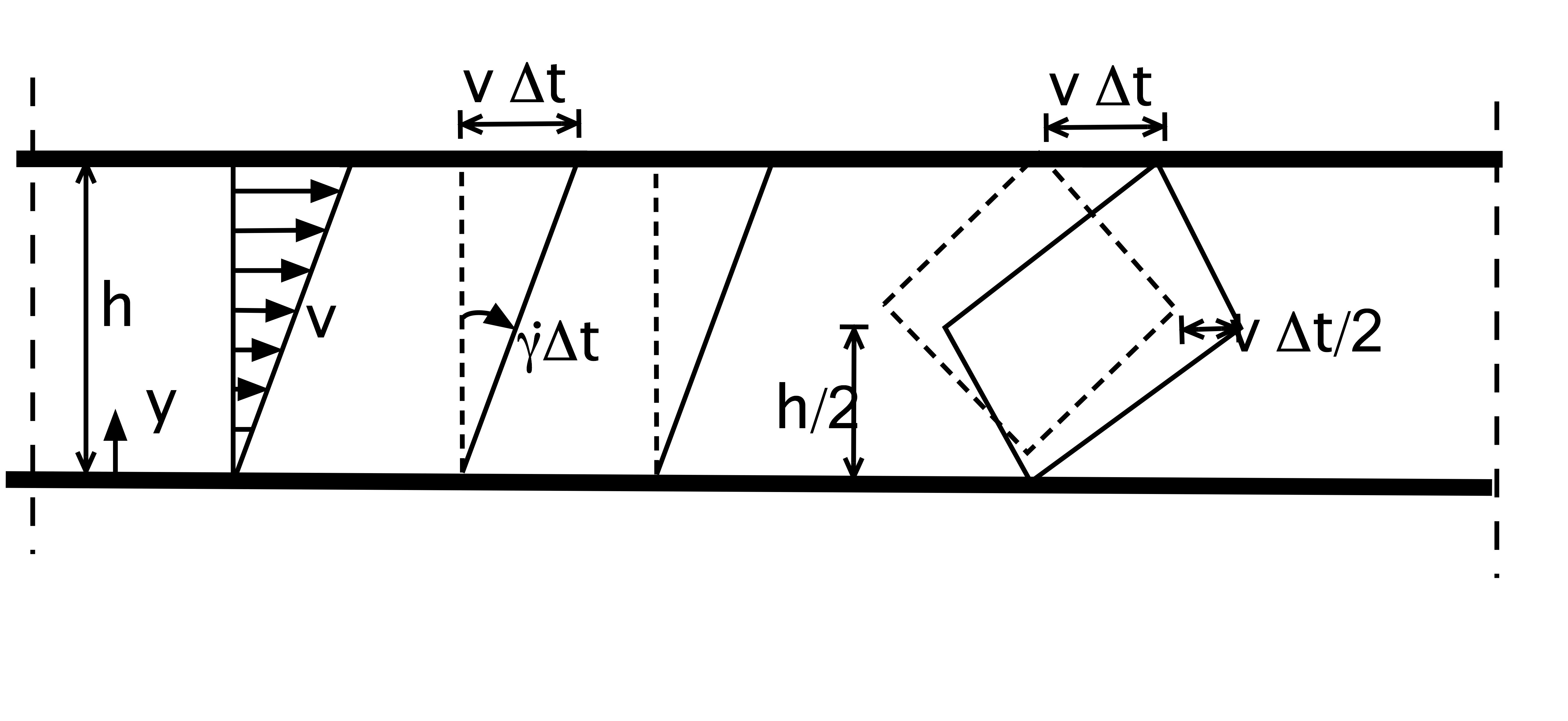
Consider fully developed fluid flow between two parallel planes, of which the lower plane is at rest, whereas the upper plane is moving with a constant velocity $ v $ parallel to the planes (see Figure 24). Assume further that the fluid particles move in straight parallel lines, and that the velocity field may be presented: $$ \begin{equation} \tag{3.92} v_x = \frac{v}{h} \, y, \qquad v_y=v_z=0 \end{equation} $$ Thus, the velocity field satisfy the no slip boundary conditions, which is used frequently in fluid dynamics. Intuitively, there might not be much in such a flow regime, normally called simple shear flow, which allude to concepts such as rotation and vorticity. However, investigation of Eq. (3.92), reveal that one component of the rate of deformation tensor $ \mathbf{D} $ is different from zero, a fact which yield a nonzero shear rate (see Eq. (3.84)): $$ \begin{equation} \tag{3.93} \dot{\gamma}_{xy} = 2 D_{xy} = \frac{v}{h}, \qquad W_{xy} = \frac{v}{2h} \end{equation} $$ and then from Eq. (3.88) we get: $$ \begin{equation} \tag{3.94} w_z \equiv \omega_z = -\frac{v}{2h} \end{equation} $$

In Figure 24, the deformation from time $ t $ to time $ t + \Delta t $ of two different fluid elements is illustrated. Fluid element 1 has been deformed with the shear rate $ \dot{\gamma}_{xy} $. Fluid element 2, was oriented with edges parallel to the principal directions of the rate of deformation tensor $ \mathbf{D} $. Fluid element 2, does not reveal the shear rates so clearly but rather show rotation with angular velocity $ w_z $. Note that the $ \epsilon_v = \text{div} \mathbf{v} = 0 $, and therefor the flow is isochoric or volume persevering. The matrices for the velocity gradient tensor $ \mathbf{L} $, the rate of deformation tensor $ \mathbf{D} $, and the rate of rotation tensor $ \mathbf{W} $ are for this simple shear flow: $$ \begin{equation} \tag{3.95} \mathbf{L} = \frac{v}{h} \left [ \begin{array}{ccc} 0 & 1 & 0 \\ 0 & 0 & 0 \\ 0 & 0 & 0 \end{array} \right ], \quad \mathbf{D} = \frac{v}{2h} \left [ \begin{array}{ccc} 0 & 1 & 0 \\ 1 & 0 & 0 \\ 0 & 0 & 0 \end{array} \right ], \quad \mathbf{W} = \frac{v}{2h} \left [ \begin{array}{ccc} 0 & 1 & 0 \\ -1 & 0 & 0 \\ 0 & 0 & 0 \end{array} \right ] \end{equation} $$

Simple shear flow is also commonly called Couette flow, after M. Couette (1890). This flow regime may be found in many applications e.g., in the flow between two cylinders with large diameter/gap ratio, of which the outer cylinder is rotating, whereas the inner cylinder is at rest.