5.5 Generalized Newtonian model
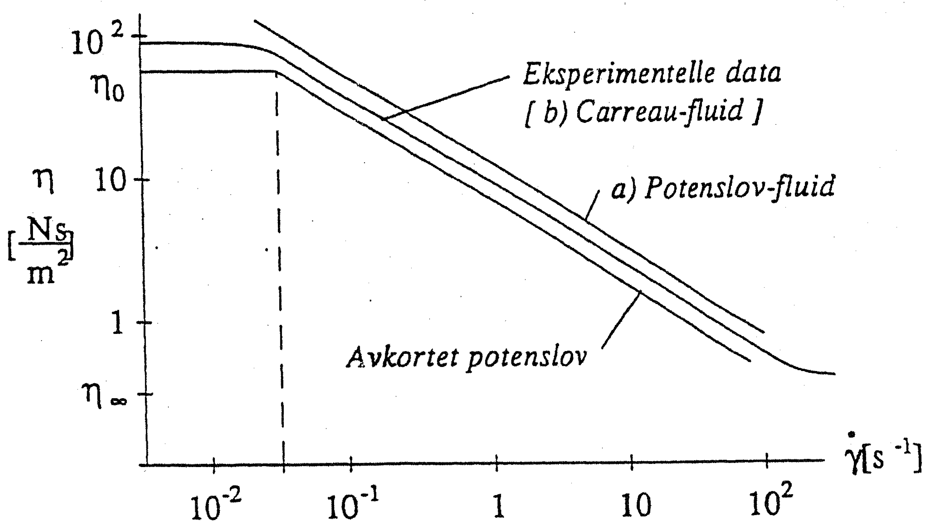
Figure 43: The viscosity function for experiments and for a Carrau-model and the power-law model .
Generalized Newtonian fluid (GNF) model for incompressible non-Newtonian fluids. $$ \begin{equation} \boldsymbol{T} = -p \boldsymbol{1} + 2 \eta \boldsymbol{D} = -p \boldsymbol{1} + \boldsymbol{\tau} \tag{5.67} \end{equation} $$
Stress deviator $$ \begin{equation} \boldsymbol{\tau} = 2 \eta \boldsymbol{D} \tag{5.68} \end{equation} $$
Viscosity function \( \eta \) $$ \begin{equation} \eta = \eta(\dot{\gamma}) \tag{5.69} \end{equation} $$
Shear measure \( \dot{\gamma} \) $$ \begin{equation} \dot{\gamma} = \sqrt{2D_{ij}D_{ij}} = 2\sqrt{-II_D} \tag{5.70} \end{equation} $$
Shear measure reduce to the strain rate for simple shear flow $$ \begin{equation} \dot{\gamma} = \partd{v_1}{x_2} \tag{5.71} \end{equation} $$
Power-law fluid. Viscosity function $$ \begin{equation} \eta = K \dot{\gamma}^{n-1} \tag{5.72} \end{equation} $$
Power-law index \( n \). Consistency parameter $$ \begin{equation} K = K_0 \exp (-A \, (\theta - \theta_0)) \tag{5.73} \end{equation} $$
Pros and cons for the power-law model: cannot fit \( \eta \) for extremal values of \( \dot{\gamma} \), however it is convenient for analytical solutions.
Most real fluids are shear thinning (\( n < 1 \)), where \( \eta \downarrow \) as \( \dot{\gamma} \uparrow \).
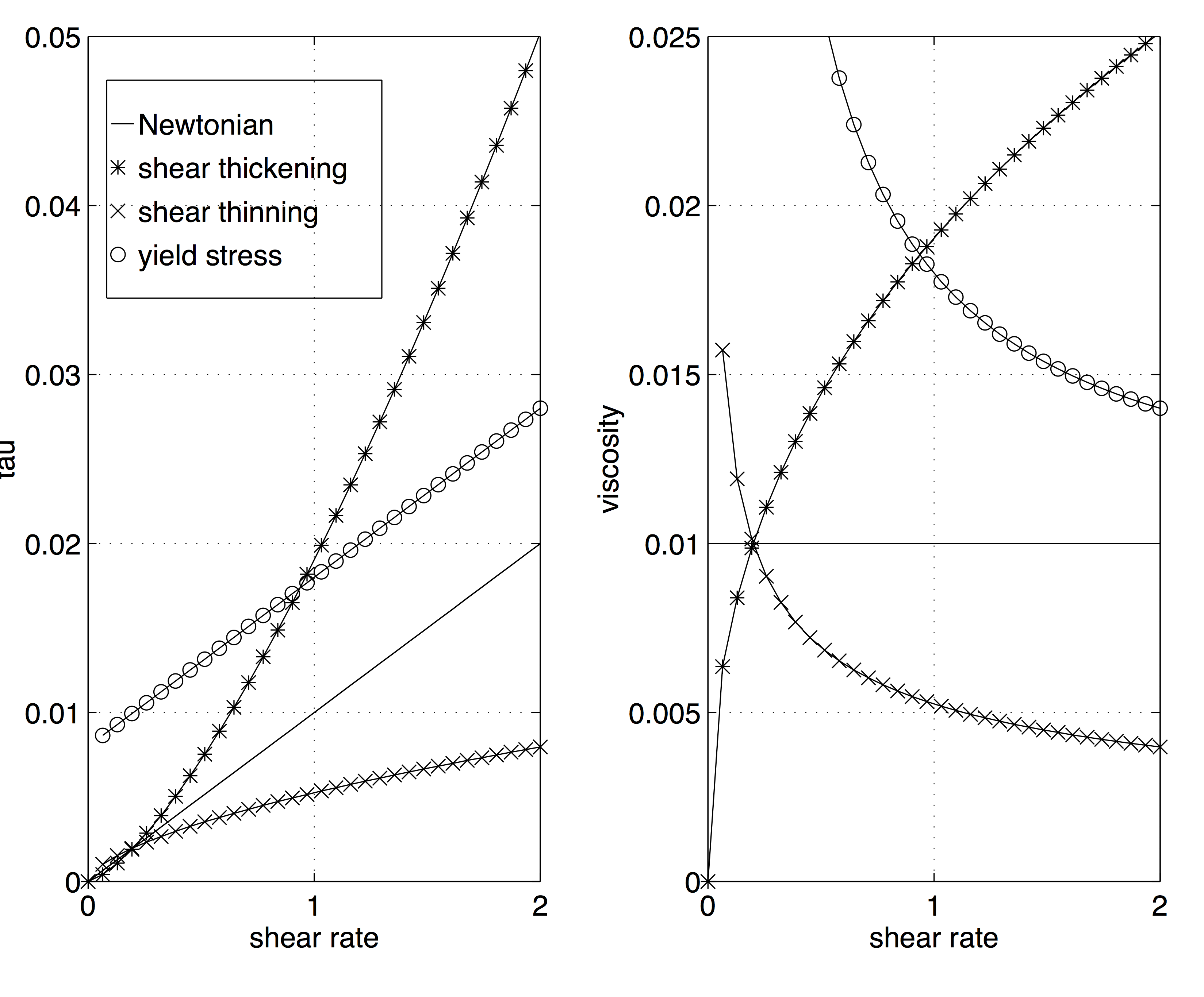
Figure 44: Shear stress as a function of shear rate (left) and the viscosity function as a function of the shear rate (right) .
Carreau-Yasuda model $$ \begin{equation} \frac{\eta -\eta_\infty}{\eta_0 -\eta_\infty} = (1+(\lambda\dot{\gamma})^2)^{n-1} \tag{5.74} \end{equation} $$
Some GNFs which fits experiments well. Casson $$ \begin{align} \tau^{\frac{1}{m}} &= \tau_0^{\frac{1}{m}} + (\eta_\infty \dot{\gamma})^{\frac{1}{m}} \tag{5.75}\\ \eta &= \eta_\infty \left [ 1 + \left (\frac{\tau_0}{\eta_\infty \dot{\gamma}} \right )^{\frac{1}{m}} \right ]^m \tag{5.76} \end{align} $$
Viscoplastic model. Bingham: \( m=1 \), Casson: \( m=2 \) The Casson-model was originally suggested for pigment/oil mixtures, but it has alos been used for blood for small \( \dot{\gamma} \). The Casson-model has Newtonian behavior as \( \dot{\gamma}\quad \uparrow \).
Cauchy equations for GNFs. Generalized Newtonian fluids $$ \begin{equation} \boldsymbol{T} = -p \boldsymbol{1} + \boldsymbol{\tau} \tag{5.77} \end{equation} $$ Cauchy's equations $$ \begin{equation} \rho \partd{\boldsymbol{v}}{t} + \rho (\boldsymbol{v} \cdot \nabla) \boldsymbol{v} = \nabla \cdot \boldsymbol{T} + \rho \boldsymbol{b} \ \tag{5.78} \end{equation} $$
Cauchy equations for generalized Newtonian fluids $$ \begin{equation} \rho \partd{\boldsymbol{v}}{t} + \rho (\boldsymbol{v} \cdot \nabla) \boldsymbol{v} = -\nabla p + \nabla \cdot \boldsymbol{\tau} + \rho \boldsymbol{b} \ \tag{5.79} \end{equation} $$
Component form $$ \begin{equation} \rho ( \partial_t v_i + v_k v_{i,k} ) = - p_{,i} + \tau_{ik,k} + \rho b_i \ \tag{5.80} \end{equation} $$
Cauchy equation in cylinder coordinates for GNF $$ \begin{align} \rho \left (\partd{v_r}{t} \right . & \left .+ v_r \partd{v_r}{r} + \frac{v_\theta}{r} \, \partd{v_r}{\theta} + v_z \partd{v_r}{z} - \frac{v_\theta^2}{r} \right ) \nonumber \\ & = -\partd{p}{r} + \frac{1}{r} \, \partd{}{r} (r \tau_{rr} ) + \frac{1}{r} \, \partd{\tau_{r\theta}}{\theta} + \partd{\tau_{rz}}{z} - \frac{\tau_{\theta\theta}}{r} + \rho b_r \tag{5.81} \end{align} $$ $$ \begin{align} \rho \left (\partd{v_\theta}{t} \right . & \left .+ v_r \partd{v_\theta}{r} + \frac{v_\theta}{r} \, \partd{v_\theta}{\theta} + v_z \partd{v_\theta}{z} + \frac{v_r v_\theta }{r} \right ) \nonumber \\ & = -\frac{1}{r}\partd{p}{\theta} + \frac{1}{r^2} \, \partd{}{r} (r^2 \tau_{r\theta} ) + \frac{1}{r} \, \partd{\tau_{\theta\theta}}{\theta} + \partd{\tau_{\theta z}}{z} + \rho b_\theta \tag{5.82} \end{align} $$ $$ \begin{align} \rho \left (\partd{v_z}{t} \right . & \left .+ v_r \partd{v_z}{r} + \frac{v_\theta}{r} \, \partd{v_z}{\theta} + v_z \partd{v_z}{z} \right ) \nonumber \\ & = -\partd{p}{z} + \frac{1}{r} \, \partd{}{r} (r \tau_{zr} ) + \frac{1}{r} \, \partd{\tau_{\theta z}}{\theta} + \partd{\tau_{zz}}{z} + \rho b_z \tag{5.83} \end{align} $$
5.5.1 Example 16: Stationary pipeflow for GNF
Simplifications: \( \boldsymbol{v} \) independent of \( z \) and \( \theta \). Deviatoric stresses are independent of \( z \) and \( \theta \).n Symmetry \( \Rightarrow \tau_{rz}=\tau_{zr} \).
Cauchy's equations in cylindrical coordinates reduce to: $$ \begin{align} 0 &= -\partd{p}{r} + \frac{1}{r} \, \partd{}{r} (r \tau_{rr} ) - \frac{\tau_{\theta\theta}}{r} \quad \mathrm{and} \quad 0 = -\frac{1}{r}\partd{p}{\theta} \notag \tag{5.84}\\ 0 &= -\partd{p}{z} + \frac{1}{r} \, \partd{}{r} (r \tau_{zr} ) \notag \tag{5.85} \end{align} $$ Constant streamwise pressure gradient (i.e., \( \partial_z p = c \)) due to $$ \begin{equation} \frac{\partial^2 p}{\partial \theta \partial z} = \frac{\partial^2 p}{\partial r \partial z} = \frac{\partial^2 p}{\partial z^2} = 0 \tag{5.86} \end{equation} $$
From simplified Cauchy equation in z-direction $$ \begin{equation} 0 = -\partd{p}{z} + \frac{1}{r} \, \partd{}{r} (r \tau_{zr} ) \tag{5.87} \end{equation} $$ we get $$ \begin{equation} \partd{}{r} (r \tau_{zr} ) = r \partd{p}{z} \tag{5.88} \end{equation} $$
By integration $$ \begin{equation} r \tau_{zr} = \frac{r^2}{2} \partd{p}{z} + C_1 \tag{5.89} \end{equation} $$
As \( \tau_{rz}(r=0) = 0 \Rightarrow C_1 = 0 \). Equilibrium equation for stationary pipeflow $$ \begin{equation} \tau_{zr} = \frac{r}{2} \partd{p}{z} \tag{5.90} \end{equation} $$
May be applied to all GNFs
5.5.2 Example 17: Power law for steady pipeflow
$$ \begin{equation} \Rightarrow \tau_{rz} = \frac{1}{2} \partd{p}{z} r \tag{5.91} \end{equation} $$ Use the power law $$ \begin{equation} \tau_{rz} = \eta \partd{v_z}{r} = K |\partd{v_z}{r}|^{n-1} \, \partd{v_z}{r} \tag{5.92} \end{equation} $$
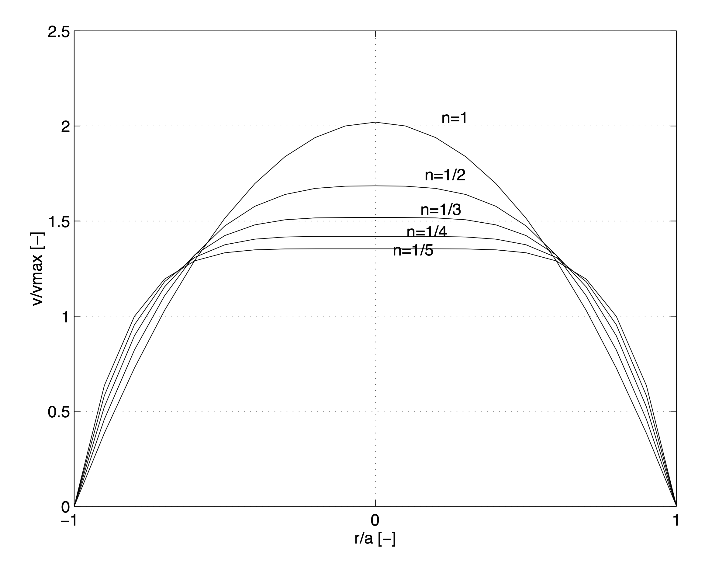
Figure 45: Velocity profiles for steady pipeflow of powerlaw fluids with different \( n \).
After subst (\( \partial_z p < 0 \)) $$ \begin{equation} \partd{v_z}{r} = -\left (\frac{1}{2K} \partd{p}{z} \, r\right )^{\frac{1}{n}} \tag{5.93} \end{equation} $$
Integrate and impose BC $$ \begin{equation} v_z = \left ( \partd{p}{z} \frac{a}{2K} \right )^{\frac{1}{n}} \frac{a}{\frac{1}{n}+1} \left ( \left ( 1 - \frac{r}{a} \right )^{\frac{1}{n} +1} \right ) \tag{5.94} \end{equation} $$
Power law and Newtonian fluid for stationary pipeflow.
Velocity profile for a power law fluid $$ \begin{equation} v_z = \left ( \partd{p}{z} \frac{a}{2K} \right )^{\frac{1}{n}} \frac{a}{\frac{1}{n}+1} \left ( 1 - \left ( \frac{r}{a} \right )^{\frac{1}{n} +1} \right ) \tag{5.95} \end{equation} $$
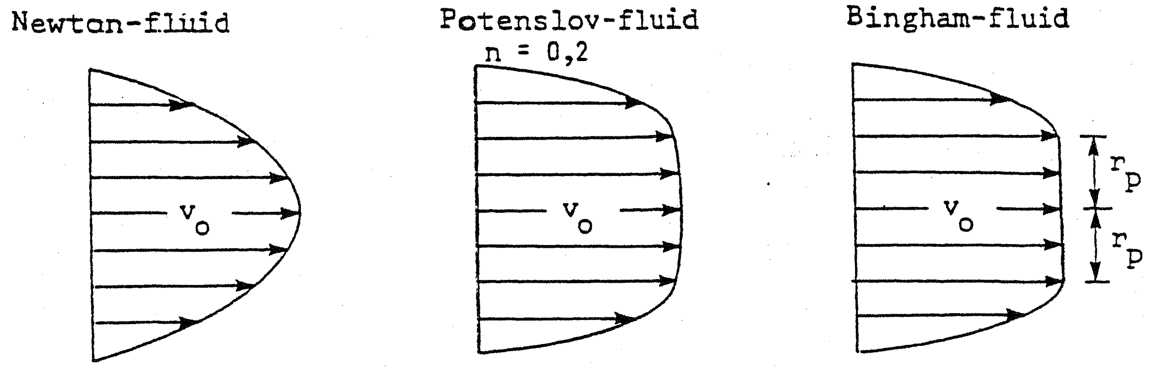
Figure 46: Pipe-flow velocity profiles for various model fluids.
Newtonian fluid (\( K=\mu \) and \( n=1 \)) in \( \eta = K \dot{\gamma}^{n-1} \) From power law velocity profile $$ \begin{align} v_z &= v_0 \left ( 1 - \left (\frac{r}{a} \right )^2 \right ) \tag{5.96}\\ v_0 &= -\frac{d^2}{16 \mu} \, \partd{p}{z} \tag{5.97} \end{align} $$ \( \Rightarrow \) power law velocity profile reduces to Newtonian expression
Velocity profiles for GNFs
Velocity profiles for Bingham fluids are obtained with similar procedure Based on equilibrium relation for stationary pipeflows Velocity profiles