4.1 Isotropic and linearly elastic materials
One may show [2] that an isotropic, linearly elastic material is completely characterized by only two independent material parameters or elasticities. Such a material is normally referred to as a Hookean material or a Hookean solid. In the following section we will derive the constitutive equations for a Hookean solid.
4.1.1 The Hookean solid
To derive the constitutive equations for a Hookean solid, consider a test beam exposed to a load of uniaxial stress, i.e., \( \sigma_1 \neq 0, \sigma_2 = \sigma_3 = 0 \). For this load the strains may be measured as: $$ \begin{equation} \tag{4.3} \epsilon_1 = \frac{\sigma_1}{\eta}, \quad \epsilon_2 = \epsilon_3 = -\nu \frac{\sigma_1}{\eta} \end{equation} $$
where \( \eta \) is the modulus of elasticity (commonly also referred to as the \( E \)-modulus) and \( \nu \) the Poisson's ratio. Now as the stress-strain relation is assumed to be linear and isotropic, the solutions of equation (4.3) may be superimposed. Consequently, a generic state of stress with three principal stresses different from zero will result in the following principal strains: $$ \begin{equation} \tag{4.4} \epsilon_1 = \frac{\sigma_1}{\eta} - \frac{\nu}{\eta} \left ( \sigma_2 + \sigma_3 \right ) = \frac{1+\nu}{\eta} \sigma_1 - \frac{\nu}{\eta} \left ( \sigma_1 + \sigma_2 + \sigma_3 \right ) \qquad \text{etc for } \epsilon_2 \text{ and } \epsilon_3 \end{equation} $$ the expression in equation (4.4) may be generalized to: $$ \begin{equation} \tag{4.5} \epsilon_i = \frac{1+\nu}{\eta} \, \sigma_i - \frac{\nu}{\eta} \, (\sigma_1 + \sigma_2 + \sigma_3) = \frac{1+\nu}{\eta} \, \sigma_i - \frac{\nu}{\eta} \,\tr \boldsymbol{T} \end{equation} $$ where the we have introduced the invariant \( \tr \boldsymbol{T} = T_{kk} =\sigma_1 + \sigma_2 + \sigma_3 \) of the stress tensor. Further, in an Ox-system with base vectors parallel to the principal directions, equation (4.5) has the matrix representation : $$ \begin{equation} \epsilon_i \, \delta_{ij} = \frac{1+\nu}{\eta} \, \sigma_i\, \delta_{ij} - \frac{\nu}{\eta} \,\tr \boldsymbol{T} \, \delta_{ij} \tag{4.6} \end{equation} $$ We may interpret equation (4.6) as a matrix representation of a tensor equation in the Ox-system with base vectors parallel to the principal directions. For an an arbitrary Ox-system, the tensor equation has the matrix representation: $$ \begin{equation} E_{ij} = \frac{1+\nu}{\eta} \,T_{ij} - \frac{\nu}{\eta} \,T_{kk} \, \delta_{ij} \tag{4.7} \end{equation} $$ The coordinate invariant tensor equation may be written: $$ \begin{equation} \tag{4.8} \boldsymbol{E} = \frac{1+\nu}{\eta} \boldsymbol{T} -\frac{\nu}{\eta} \tr \boldsymbol{T} \, \boldsymbol{1} \end{equation} $$ The equations (4.7) and (4.8) are normally denoted the generalized Hooke's law and represent the constitutive equations for a Hookean material, i.e., an isotropic, linearly elastic material. Equivalent representations of the generalized Hooke's law, may be formulated with stress on the left hand side of the equations: $$ \begin{align} T_{ij} &= \frac{\eta}{1+\nu} \, \left ( E_{ij} + \frac{\nu}{1-2\nu} \, E_{kk} \, \delta_{ij} \right ) \tag{4.9}\\ \boldsymbol{T} &= \frac{\eta}{1+\nu} \, \left ( \boldsymbol{E} + \frac{\nu}{1-2\nu} \, E_{kk} \, \boldsymbol{1} \right ) \tag{4.10} \end{align} $$
Keep in mind that a Hookean material is completely characterized by two material parameters (\( \eta \) and \( \nu \)). Observe from equations (4.7) and (4.9) and (4.10) that normal stresses (\ie \( T_{ii} \) with no summation) only result in longitudinal strains (\ie \( E_{ii} \) with no summation), and vice versa. Similarly, shear stresses (\( T_{ij} \)) only produce shear strains (\( E_{ij} \)). These relations are not valid in general for anisotropic materials.
For shear stresses and shear strains (i.e., when \( i \neq j \)), the last term of equation (4.9) drops out and one may write: $$ \begin{equation} \tag{4.11} T_{ij} = 2 \mu E_{ij} = \mu \gamma_{ij}, \quad i \neq j \end{equation} $$ where we have introduced the shear modulus as: $$ \begin{equation} \mu = \frac{\eta}{2(1+\nu)} \tag{4.12} \end{equation} $$
The shear modulus may thus be thought of as an E-modulus for shear stress/strain conditions, such as torsion of a cylinder.
A relation between the volumetric \( \varepsilon_v \) strain and the stresses may be found by computing the trace of equation (4.7): $$ \begin{equation} \tag{4.13} \varepsilon_v = E_{ii} = \frac{1+\nu}{\eta} \,T_{ii} - \frac{\nu}{\eta} \,T_{kk} \, \delta_{ii} = \frac{1-2\nu}{\eta} T_{ii} \end{equation} $$ By introducing the bulk modulus \( \kappa \): $$ \begin{equation} \tag{4.14} \kappa = \frac{\eta}{3\, (1-2\nu)} \end{equation} $$
and the mean stress as: $$ \begin{equation} \tag{4.15} \sigma^0 = \frac{1}{3} T_{ii} \end{equation} $$
equation (4.13) may be presented in the more compact form: $$ \begin{equation} \tag{4.16} \sigma^0 = \frac{1}{\kappa} \varepsilon_v \end{equation} $$ Fluids are generally considered to be linearly elastic materials when sound wave propagation is to be analyzed. The bulk modulus for water is \( \kappa = 2.1\, GPa \), for mercury \( \kappa = 27 \, GPa \), and for alcohol \( \kappa = 0.91 \, GPa \). From equation (4.14), we see that \( \nu > 1/2 \), would give unphysical values for the bulk modulus \( \kappa < 0 \), as in such a situation the volume of a material would increase when being exposed to an isotropic pressure. Further, the Poissons ratio is expected to be positive \( \nu \leq 0 \), as \( \nu < 0 \) corresponds to a material which expand in the direction perpendiualr to the stress direction, in the case of uniaxial stretch. Thus, we expect: $$ \begin{equation} \tag{4.17} 0 \leq \nu \leq 0.5 \end{equation} $$ Among real materials, rubber is considered to be almost incompressible with \( \nu = 0.49 \), whereas cork represents the other extreme with \( \nu \approx 0 \). This property for cork is indeed a desired property whenever one is trying to cork a bottle.
A simple form for Hooke's law may be obtained by splitting the stress and strain tensors in isotropic and deviatoric parts: $$ \begin{equation} T_{ij} = T^0_{ij} + T'_{ij} \quad \text{ and } \quad E_{ij} = E^0_{ij} + E'_{ij} \tag{4.18} \end{equation} $$ where 0-superscripts denote the isotropic tensors: $$ \begin{equation} T^0_{ij} = \sigma^0 \, \delta_{ij} \quad \text{ and } \quad E^0_{ij} = \frac{1}{3} \varepsilon_v \, \delta_{ij} = \frac{1}{3} E_{kk} \, \delta_{ij} \tag{4.19} \end{equation} $$ Substitution of equation (4.19) into equation (4.7) or (4.9) the yields the simple forms for isotropic or deviatoric loads repsectively: $$ \begin{equation} T^0_{ij} = 3 \kappa E^0_{ij} \quad \text{and} \quad T'_{ij} = 2 \mu E'_{ij} \tag{4.20} \end{equation} $$ By summation of the two equations in (4.20) we get: $$ \begin{align} T_{ij} = T'_{ij} + T^0_{ij} &= 2 \mu E'_{ij} + 3 \kappa E^0_{ij} \tag{4.21}\\ & = 2 \mu (E_{ij}-E^0_{ij}) + \kappa E_{kk} \delta_{ij} \tag{4.22} \end{align} $$
where we use the trace of the strain tensor \( E_{kk} \) in equation (4.19) to eliminate expressions with the isotropic strain tensor \( E^0 \). A final elimination of \( E^0 \) yields yet another formulation of a Hookean material: $$ \begin{equation} T_{ij} = 2 \mu E_{ij} + \left (\kappa -\frac{2\mu}{3} \right ) E_{kk} \delta_{ij} \tag{4.23} \end{equation} $$
For an incompressible Hookean material the volume does not change (\ie \( \varepsilon_v = 0 \)), and the mean stress \( \sigma^0=T_{kk}/3 \) can not be determined from Hooke's law. For such materials the constitutive equation (4.9) is normally reformulated as: $$ \begin{equation} \boldsymbol{T} = -p \, \boldsymbol{1} + 2\mu \, \boldsymbol{E} \tag{4.24} \end{equation} $$ which on component form has the representation: $$ \begin{equation} T_{ij} = -p \, \delta_{ij} + 2 \mu E_{ij} \tag{4.25} \end{equation} $$ where \( p=p(\boldsymbol{r},t) \) is an unknown pressure (or positive normal stress) which can only be determined from the equations of motion and the boundary conditions.
4.1.2 Navier equations
In this section we use the Cauchy equations (2.89) and the constitutive equations for a Hookean material (4.7), to derive the governing Navier equations for a Hookean material.
For convenience we introduce the shear modulus: $$ \begin{equation} \mu = \frac{\eta}{2(1+\nu)} \tag{4.26} \end{equation} $$ and multiply (4.7) with \( \frac{2(1+\nu)}{\eta}=1/\mu \), and differentiate with respect to \( x_k \) to obtain an expression for the divergence of the stress tensor: $$ \begin{align} \frac{1}{\mu}\, T_{ik,k}&=u_{i,kk}+\underbrace{u_{k,ik}}_{=u_{k,ki}}+\frac{2\nu}{1-2\nu}\underbrace{u_{l,lk}\delta_{ik}}_{=u_{l,li}=u_{k,ki}} \tag{4.27}\\ &=u_{i,kk}+\left (1+\frac{2\nu}{1-2\nu} \right )u_{k,ki} \tag{4.28}\\ \frac{1}{\mu}T_{ik,k}&=u_{i,kk}+\frac{1}{1-2\nu}u_{k,ki} \tag{4.29} \end{align} $$
The expression for the divergence of the stress tensor (4.29) may the be substituted into Cauchy equations (2.89) to give the: Navier equations: $$ \begin{align} u_{i,kk}+\frac{1}{1-2\nu}u_{k,ki}+\frac{\rho}{\mu} \, (b_i-\ddot{u}_i)=0 \tag{4.30} \end{align} $$ which constitute a system of partial differential equations which may be solved along with appropriate boundary conditions.
4.1.3 2D theory of elasticity
The general equations for Hookean materials have solutions only in a few special and simple cases. However, in many problems of practical interest we may introduce simplifications, either with respect to the state of stress or the state of strain, in such a way that useful solutions may be found analytically.
4.1.3.1 Plane stress
Figure 28: A thin walled spherical shell of steel.
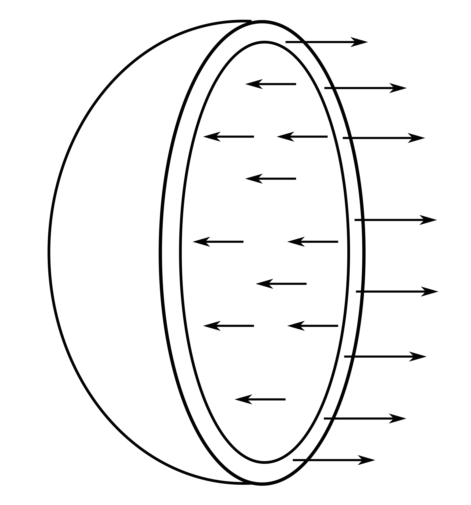
For a plane stress assumption to be valid, we normally consider a thin structure of some kind such as a thin plate or a thin sphere (see figure 28) loaded by body forces \( \boldsymbol{b} \) and contact forces \( \boldsymbol{t} \) on the surface \( A \) of the structure such that: $$ \begin{align} b_{\alpha} &= b_{\alpha} (x_1,x_2,t), \qquad b_3 = 0 \tag{4.31}\\ t_{\alpha} &= t_{\alpha} (x_1,x_2,t), \qquad t_3 = 0 \tag{4.32} \end{align} $$ In such a situation one may approximate the state of stress as a state of plane stress, which may be represented mathematically: $$ \begin{equation} T_{i3} = 0 \qquad \text{and} \qquad T_{\alpha\beta}=T_{\alpha\beta}(x_1,x_2,t) \tag{4.33} \end{equation} $$ The validity of the plane stress assumption will normally rest on the condition that the wall thickness \( h \) of the structure is much smaller than the a characteristic dimension, such as the diameter, of the structure.
The govering equations for a thin walled structure in plane stress are Cauchy's equations of motion (see (2.89)) $$ \begin{equation} \rho \ddot{\boldsymbol{u}} = \nabla \cdot \boldsymbol{T} + \rho \boldsymbol{b} \Leftrightarrow \rho \ddot{u}_{\alpha} = T_{\alpha\beta,\beta} + \rho b_{\alpha} \tag{4.34} \end{equation} $$
Note that we have used the second material derivative of the displacement for the acceleration, which in turn will be represented by the second partial derivative of \( \mathbf{u} \) with respect to time, while assumping small deformations: $$ \begin{equation} \ddot{u}_{\alpha} = \partdd{u _{\alpha} }{t} \tag{4.35} \end{equation} $$ Further, we assume that the material may be represented with Hooke's law for plane stress (see Exercise 1: The generalized Hooke's law): $$ \begin{equation} T_{\alpha\beta} = 2 \mu \left ( E_{\alpha\beta} + \frac{\nu}{1-\nu} \, E_{\rho\rho} \delta_{\alpha\beta} \right ), \quad 2\mu = \frac{\eta}{1+\nu} \tag{4.36} \end{equation} $$ where the shear modulus \( \mu \) has been introduced conventionally.
As for the generic Hookean law the plane stress version may be written with the strains on the right hand side: $$ \begin{equation} E_{\alpha\beta} = \frac{1}{2\mu} \, \left ( T_{\alpha\beta} - \frac{\nu}{1+\nu} \, T_{\rho\rho} \delta_{\alpha\beta} \right ), \qquad E_{33} = - \frac{\nu}{\eta} T_{\rho\rho} \tag{4.37} \end{equation} $$ Note that the strain has three components even though the stress is planar, due to the conservation of mass.
For small displacements (see equation (3.48) ) the Green strain tensor reduce to: $$ \begin{equation} E_{\alpha\beta} = \frac{1}{2} \left ( u_{\alpha,\beta} + u_{\beta,\alpha} \right ) \tag{4.38} \end{equation} $$ which explicitly relates the strain tensor to displacements. Together, the equations (4.34), (4.36), and (4.38) constitute 8 equations (2+3+3), for what may be regarded as 8 unknown fuctions \( T_{\alpha\beta} \) (3 components), \( E_{\alpha\beta} \) (3 components), and \( u_\alpha \) (2 components). Thus, these equations represent a closed system of partial differential equations. As there is a linear relation between stresses and strains (displacements), one may choose either stresses or displacements as the primary function when representing the resulting partial differential equations.
By substitution of the plane stress version of Hooke's law as given by equation (4.36), and equation (4.38), into the Cauchy equations (4.34) (see Exercise 1: The generalized Hooke's law) we get a displacement version of the:
Navier equations for plane stress: $$ \begin{equation} u_{\alpha,\beta\beta} + \frac{1+\nu}{1-\nu} \, u_{\beta,\beta\alpha} + \frac{\rho}{\mu} \left (b_{\alpha} - \ddot{u}_{\alpha} \right )= 0 \tag{4.39} \end{equation} $$ With these substitutions, both stresses and strains have been eliminated, while the displacements remain as the only two unknowns in the two equations of motion in (4.39).
To complete the solution to the problem, boundary conditions must be provided. Normally, one assume that contact forces, or stresses/tractions, are imposed on a part \( A_\sigma \) of the surface of the structure, while displacements are imposed on the remaining part \( A_u = A-A_\sigma \), which may be represented mathematically: $$ \begin{align} t_{\alpha} &= t_{\alpha}^*, \quad \text{on} \; A_{\sigma} \tag{4.40} \\ u_{\alpha} &= u_{\alpha}^*, \quad \text{on} \; A_{u} \tag{4.41} \end{align} $$
Having found the solution of the Navier equations (4.39), typically by means of some numerical method, for the imposed boundary conditions (4.40) and (4.41), one may compute the stresses for the constitutive relation in equation (4.36).
4.1.4 Example 9: Spherical shell of steel
We consider a thin walled spherical shell of steel with diameter \( d_0=2000 \) mm (Figure 28) and wall thickness \( t_0 = 5 \) mm at zero transmural pressure. The sphere is then inflated with a transmural pressure of \( p=1.5 \) MPa. We want to find the change in diameter and wall thickness due to the imposed load.
From the stress analysis in example 2.5.4 Example 6: Biaxial state of stress for thin-walled structures we get expressions for the wall stresses in the \( \theta \)- and \( \phi \)-directions, which are principal stress directions , from (2.164): $$ \begin{equation} \sigma_{\phi} = \sigma_{\theta} = \sigma =\frac{1}{2} \frac{r}{t} p = \frac{1}{2 \,(5\cdot 10^{-3})} \, 1.5\cdot 10^6 = 150 \; \hbox{MPa} \tag{4.42} \end{equation} $$ The stress in the radial direction must be in the order of \( p \), \ie \( \sigma_r \propto p \ll \sigma \Rightarrow \sigma_r \approx 0 \). Steel is assumed to be a Hookean material with \( \eta= 210 \;\hbox{GPa} \) and \( \nu=0.3 \) and strains resulting from the imposed stresses may either be calculated from Hooke's law in (4.7) or from the tailor made version of Hooke's law for plane stress in equation (4.37). In the azimuthal direction, we denote the coordinate strain by \( \varepsilon_{\theta} \) and get from (4.7): $$ \begin{align} \varepsilon_{\theta} & = E_{11} = \frac{1+\nu}{\eta} \sigma_{\theta} - \frac{\nu}{\eta} \left (\sigma_{\theta} + \sigma_{\phi} \right ) = \frac{1-\nu}{\eta} \, \sigma \nonumber \\ &= \frac{1-0.3}{210\cdot 10^9} \, \cdot 150 \cdot 10^6 = 0.5 \cdot 10^{-3} \tag{4.43} \end{align} $$ From the Hooke's law for plane stress in equation (4.37) we get the same expression as in equation (4.43): $$ \begin{equation} \varepsilon_\theta = \frac{1+\nu}{\eta} \left (\sigma_\theta - \frac{\nu}{1+\nu} (\sigma_\theta + \sigma_\phi ) \right ) = \frac{1-\nu}{\eta} \, \sigma \tag{4.44} \end{equation} $$ The azimuthal strain \( \varepsilon_{\theta} \) is related with changes in the diameter in the following manner: $$ \begin{align} \varepsilon_{\theta} & = \frac{\pi d - \pi d_0}{\pi d_0} = \frac{d-d_0}{d_0} = \frac{\Delta d}{d_0} \tag{4.45} \end{align} $$ Thus, the change in diameter due to the imposed pressure load is: $$ \begin{equation} \Delta d = \varepsilon_{\theta} \, d_0 = 0.5 \cdot 10^{-3}\, 2000 = 1 \, \mathrm{mm} \tag{4.46} \end{equation} $$ The strain in the radial direction \( \varepsilon_{r} \) is also readily obtained from (4.7) or from the planar stress version in equation (4.37): $$ \begin{align} \varepsilon_{r} & = E_{33} = - \frac{\nu}{\eta} \left (\sigma_{\theta} + \sigma_{\phi} \right ) = \frac{-2\nu}{\eta} \, \sigma \nonumber \\ &= \frac{-0.6}{210\cdot 10^9} \, \cdot 150 \cdot 10^6 = -\frac{3}{7} \cdot 10^{-3} \tag{4.47} \end{align} $$ and is related with changes in wall thickness: $$ \begin{align} \varepsilon_r & = \frac{t-t_0}{t_0} = \frac{\Delta t}{t_0} \tag{4.48} \end{align} $$ Consequently, the change in wall thickness is negative and given by: $$ \begin{equation} \Delta t = \varepsilon_r t_0 = -\frac{3}{7} \cdot 10^{-3} \approx -2.1 \cdot 10^{-3} \mathrm{mm} \tag{4.49} \end{equation} $$
4.1.5 Plane displacement
For plane displacements we assume that the displacement vector have only to components which in tur are functions of the two coordinate direction in which the displacements are taking place : $$ \begin{align} u_{\alpha} = u_{\alpha}(x_1,x_2,t), \quad u_3 = 0 \tag{4.50} \end{align} $$
Consequently, we have \( E_{i3} = 1/2 (u_{i,3} + u_{3,i}) = 0 \) and the strain tensor reduces to: $$ \begin{align} E_{\alpha \beta} = \frac{1}{2} \, (u_{\alpha, \beta} + u_{\beta, \alpha}), \quad E_{i3} = 0 \tag{4.51} \end{align} $$
One may show that in the case of plane displacements given by (4.51) the generic Navier equations (4.30) reduce to: $$ \begin{align} u_{\alpha,\beta\beta} + \frac{1}{1-2\mu} \, u_{\beta, \alpha \beta} + \frac{\rho}{\mu} (b_{\alpha} - \ddot{u}_{\alpha} )= 0 \tag{4.52} \end{align} $$ i.e., the only diffenrences from equations (4.30) are that the sums are trucanted to constitute only two elements.
Further, we assume that the displacements are axisymmetric, which in mathematical terms means: $$ \begin{equation} u_r = u_r(r), \quad u_{\theta} = u_{\theta}(r) \tag{4.53} \end{equation} $$ and consequently: $$ \begin{equation} u_{\beta, \beta\alpha} = u_{\alpha,\beta\beta} = \left \{ \begin{array}{cc} 0 & \alpha = \theta \\ \D \partdd{u_r}{r} & \alpha = r \end{array} \right . \tag{4.54} \end{equation} $$ Substitution of (4.54) into (4.52) yields: $$ \begin{align} \frac{2\, (1-\mu)}{1-2\mu} \, u_{\beta,\beta \alpha} + \frac{\rho}{\mu} (b_{\alpha} - \ddot{u}_{\alpha} )= 0 \tag{4.55} \end{align} $$
For longitudinal strains and axisymmetric displacements: $$ \begin{align} \epsilon_r &= \frac{du}{dr}, \qquad \epsilon_{\theta} = \frac{l-l_0}{l_0} = \frac{2\pi (r+u) - 2\pi r}{2\pi r} = \frac{u}{r} \nonumber \\ \epsilon_A &= \epsilon_r + \epsilon_{\theta} = \frac{du}{dr} + \frac{u}{r} = \frac{1}{r} \frac{d(ur)}{dr} \tag{4.56} \end{align} $$
Figure 29: Radial and cicumferential strains for plane displacement.
By differentiation of (4.56) we get: $$ \begin{align} \epsilon_{A,\alpha} = u_{\beta, \beta \alpha} \Rightarrow \epsilon_{A,r} = \frac{d}{dr} \left ( \frac{1}{r} \frac{d(ur)}{dr} \right ) \tag{4.57} \end{align} $$
If we neglect body forces and intertia, we get by substitution of (4.57) into (4.55): $$ \begin{align} \frac{d}{dr} \left ( \frac{1}{r} \frac{d(ur)}{dr} \right ) = 0 \tag{4.58} \end{align} $$ Thick walled cylinder with internal and external pressures $$ \begin{align} u(r) =& \frac{1}{2\eta}\, \frac{a}{1-(a/b)^2} \left [ \left (\frac{a}{r} + (1-2\nu) \left (\frac{a}{b}\right )^2 \, \frac{r}{a} \right ) p - \left (\frac{a}{r} + (1-2\nu) \, \frac{r}{a} \right )q \right ] \tag{4.59}\\ \sigma_r(r) =& \frac{2\mu}{1-\nu} \, \left ( \frac{du}{dr} + \nu \frac{u}{r} \right ) \tag{4.60}\\ \sigma_{\theta}(r) = &\frac{2\mu}{1-\nu} \, \left ( \frac{u}{r} + \nu \frac{du}{dr} \right ) \tag{4.61} \end{align} $$
Figure 30: Solutions for thick walled cylinder with internal and external pressures
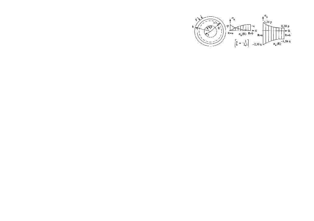
4.1.6 Example 10: Plane displacements for a thick walled cylinder
The assumption of plane displacements may be expressed mathematically as: $$ \begin{equation} u_\alpha = u_\alpha(x_1,x_2,t), \quad u_3 = 0 \tag{4.62} \end{equation} $$ The Green deformation tensor for small deformations (see Equation (3.48)) reduce to: $$ \begin{equation} \tag{4.63} E_{\alpha \, \beta} = \frac{1}{2} \left ( u_{\alpha, \beta} + u_{\beta, \alpha} \right ), \quad E_{i3} = 0 \end{equation} $$
The components of the stress tensor for a Hookean material Equation (4.9) corresponding to the directions of non-zero displacements may the be represented:
based on Equation (4.63) and by using the shear modulus in Equation (4.26).
2: Repeated Greek indices imples sum from 1 to 2.
3: Engineering notation is used as stresses are principal stresses.