2.3 Equations of motion
As Newton's laws for the motion of mass particles cannot be transferred directly to a body of continuously distributed matter, Euler's two axioms are postulated in Continuum Mechanics: Law of balance of linear momentum and Law of balance of angular momentum. The axioms will be presented in mathematical terms in this section, and based on these axioms the equations of motion will be derived. We will also show that, based on the two axioms, the equations of motion for the center of mass (to be defined) of a body is identical with Newton's second law. One may also show that Newton's third law of action and reaction also follow from the two axioms (see section 3.2.2 [2]).
Note that the relation in (2.42), between the rate of change of the extensive linear momentum \( \dot{\mathbf{P}} \), and the integral of the rate of change of the intensive specific linear momentum \( \dot{\mathbf{v}} \), follow from (2.34).
Figure 3: Body forces \( \mathbf{b} \) and surface forces \( \mathbf{t} \) on a volume \( V \) with surface area \( A \).
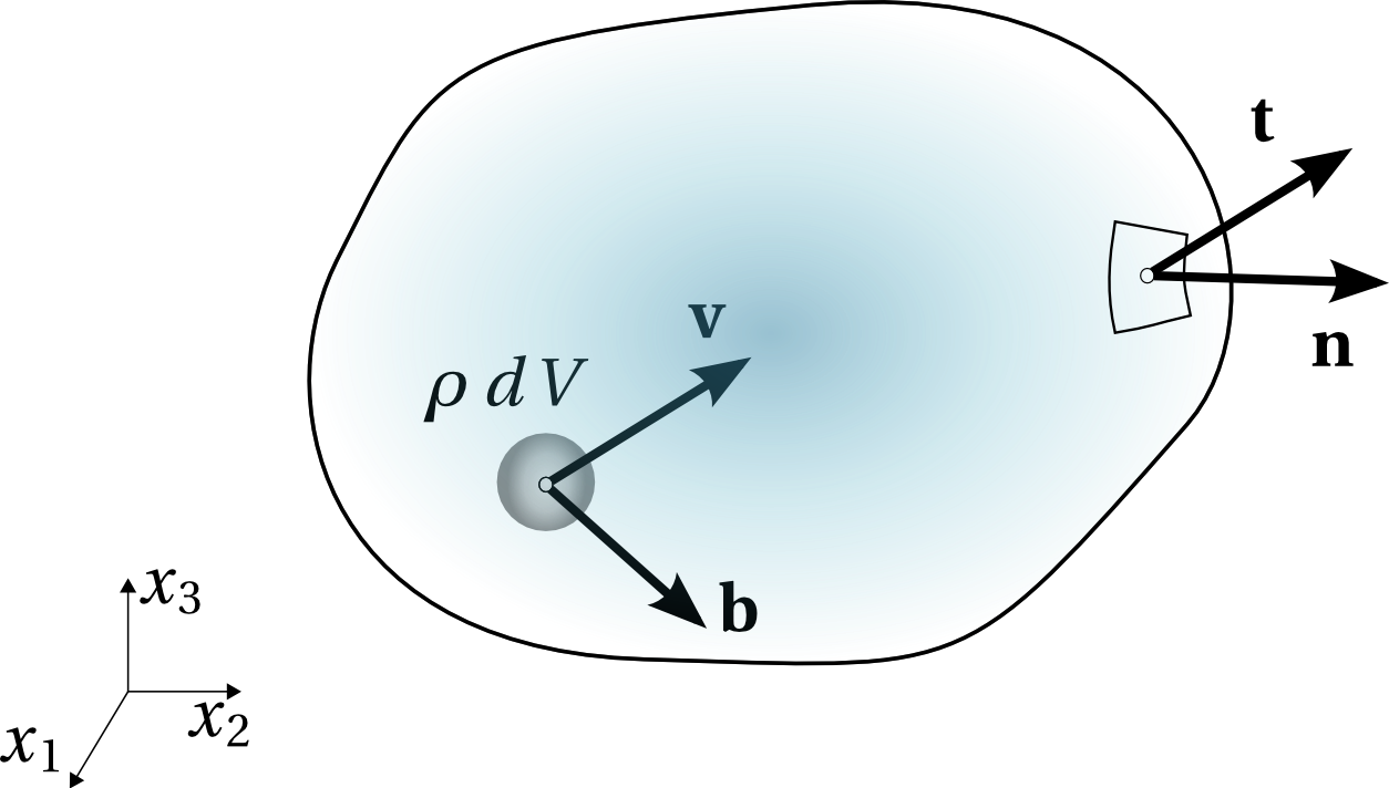
As we in applications of continuum mechanics are concerned with how strains and stresses are distributed throughout the body of interest, the forces of (2.42) must be represented as intensive quantities too. This is due to that we will present the final governing equations as differential equations rather than integral equations. The body of interest (see Figure 3) is assumed to be acted upon by two types of forces: body force \( \mathbf{b} \) per unit mass, and contact force \( \mathbf{t} \) per unit area. Consequently, the extensive resultant force is related with its intensive components by: $$ \begin{equation} \mathbf{f} = \int_A \mathbf{t} \, dA + \int_V \mathbf{b} \, \rho \, dV \tag{2.43} \end{equation} $$ By substitution of (2.43) in (2.42) an integrated representation of the the law of balance of linear momentum may be found:
Law of balance of linear momentum integral formulation $$ \begin{equation} \int_V \dot{\mathbf{v}} \rho \, dV = \int_A \mathbf{t} \, dA + \int_V \mathbf{b} \, \rho \, dV \tag{2.44} \end{equation} $$
Balance of linear momentum and Newton's second law To see how (2.42) is related with Newton's second law, we introduce the center of mass: $$ \begin{equation} \mathbf{r}_C = \frac{1}{m} \, \int_V \mathbf{r} \, \rho \, dV \tag{2.45} \end{equation} $$ Further, the velocity and acceleration of the center of mass is defined in a logical manner: $$ \begin{align} \mathbf{v}_C &= \frac{1}{m} \, \int_V \mathbf{v} \, \rho \, dV = \frac{1}{m} \, \int_V \dot{\mathbf{r}} \, \rho \, dV =\dot{\mathbf{r}}_C \tag{2.46}\\ \mathbf{a}_C &=\dot{\mathbf{v}}_C = \frac{1}{m} \, \int_V \dot{\mathbf{v}} \, \rho \, dV = \ddot{\mathbf{r}}_C = \frac{1}{m} \, \int_V \mathbf{a} \, \rho \, dV \tag{2.47} \end{align} $$
Substitution of (2.47) in (2.42) yields: $$ \begin{equation} \mathbf{f} = m \mathbf{a}_C \tag{2.48} \end{equation} $$ which is Newton's second law for the center of mass and an extensive representation of (2.44).
To express this axiom in a more useful way mathematically, we must find the intensive expressions for its constituents. The resultant moment \( \mathbf{m}_0 \) has contributions both from surface forces and body forces: $$ \begin{equation} \mathbf{m}_0 = \int_A \mathbf{r \times t}\, dA + \int_V \mathbf{r \times b} \, \rho \, dV \tag{2.50} \end{equation} $$ The angular momentum is given by: $$ \begin{equation} \mathbf{l}_0 = \int_V \mathbf{r \times v} \rho \, dV \tag{2.51} \end{equation} $$ and the rate of change of the angular momentum may be show to be: $$ \begin{equation} \dot{\mathbf{l}}_0 = \int_V \mathbf{r \times \dot{v}} \rho \, dV \tag{2.52} \end{equation} $$ The result in (2.52) follow from (2.34) and from by the expansion: $$ \begin{equation} \dot{\mathbf{r \times v}} = \dot{\mathbf{r}} \times \mathbf{v} + \mathbf{r} \times \dot{\mathbf{v}} \tag{2.53} \end{equation} $$ The first term in (2.53) vanishes due to: $$ \begin{equation} \dot{\mathbf{r}} = \mathbf{v} \quad \mathrm{and} \quad \mathbf{v \times v} = 0 \tag{2.54} \end{equation} $$
An equivalent representation of the law of balance of angular momentum is then found by substitution of Eqs. (2.52) and (2.50) in (2.49):
Law of balance of angular momentum integral formulation $$ \begin{equation} \int_V \mathbf{r \times \dot{v}} \rho \, dV = \int_A \mathbf{r \times t}\, dA + \int_V \mathbf{r \times b} \, \rho \, dV \tag{2.55} \end{equation} $$
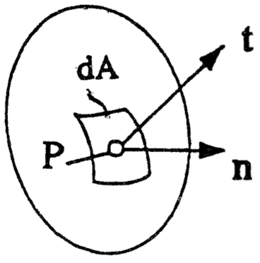
Figure 4: Surface stress \( \mathbf{t} \) on surface with normal vector \( \mathbf{n} \).
2.3.1 Coordinate stresses
In Figure 4 the stress vector \( \mathbf{t} \) is shown on a surface with orientation \( \mathbf{n} \) in a particle (or point) P. This surface may either be the physical surface or an arbitrary oriented surface within a body of interest. In an orthogonal coordinate system Ox with orthogonal unit vectors \( \mathbf{e}_i \), the vectors \( \mathbf{t} \) and \( \mathbf{n} \) are expressed as a sum their components \( t_i \) and \( n_i \), respectively (remember Einsteins's summation convention): $$ \begin{equation} \mathbf{t} = t_i \; \mathbf{e}_i \qquad \text{and} \qquad \mathbf{n} = n_k \; \mathbf{e}_k \tag{2.56} \end{equation} $$
Now, let us consider the situation illustrated in Figure 5, in which we have oriented three orthogonal planes through the point P, with unit normals \( \mathbf{e}_k \). On each of the planes \( \mathbf{e}_k \), a stress vector \( \mathbf{t}_k \) acts, with \( k=1\ldots 3 \).
In the same way as in (2.56), the three \( \mathbf{t}_k \) vectors may be expressed by their components, $$ \begin{equation} \mathbf{t}_k = T_{ik} \mathbf{e}_i \quad \Leftrightarrow \quad \mathbf{e}_i \cdot \mathbf{t}_k = T_{ik} \tag{2.57} \end{equation} $$ for an arbitrary \( k \), where we have introduced \( T_{ik} \) which denotes the coordinate stresses in the particle P. The coordinate stresses \( T_{ik} \) are elements of the stress matrix \( T \). in P with respect to the coordinate system Ox. And as \( T_{ik} \), represents, the components in Ox of the three \( \mathbf{t}_k \) on three orthogonal surfaces, it \( T_{ik} \) represents the complete stress situation in the particle P.
Figure 5: Stresses and coordinate stresses on three orthogonal surfaces.
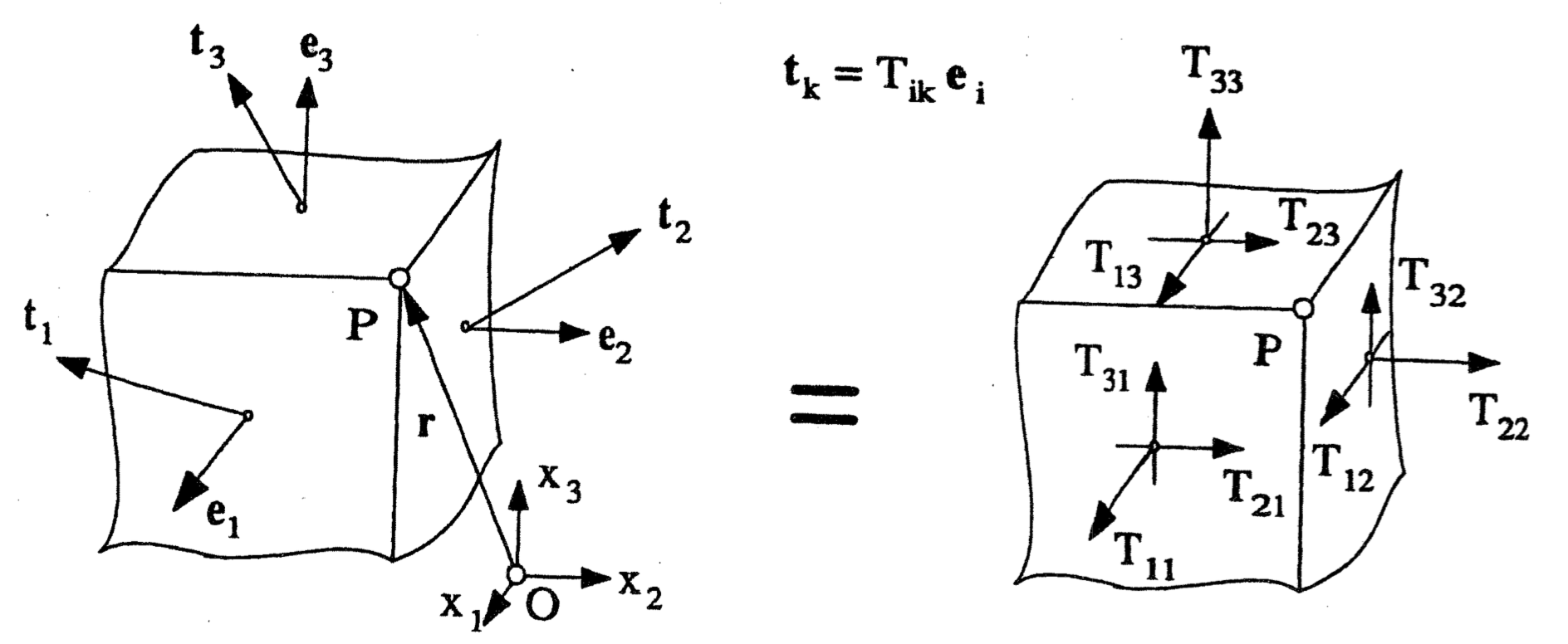
The coordinate stresses \( T_{11} \), \( T_{22} \), \( T_{33} \), are denoted normal stresses, whereas \( T_{ik} \), when \( i\neq k \), are denoted shear stresses. In this presentation, first index i refers to the direction of the of the stress, while the second index k refers to the face, with normal vector \( \mathbf{e}_k \), on which the stress \( T_{ik} \) acts. The order or meaning of the indices are often reversed in the literature. However, the laws of balance of angular/linear momentum will later be used be used to show that the stress matrix is symmetric when only body forces \( \mathbf{b} \) and contact forces \( \mathbf{t} \) are considered (see (2.93). $$ \begin{equation} T_{ij} = T_{ji} \quad \Leftrightarrow \quad \mathbf{T}^T = \mathbf{T} \tag{2.58} \end{equation} $$
Thus, the order of the indices is normally not important, and one may use the mnemonic: "First Face Second Stress" to remember the meaning of the indices.
Figure 6: Coordinate stresses on a surface parallel with \( \mathbf{e}_2 \).
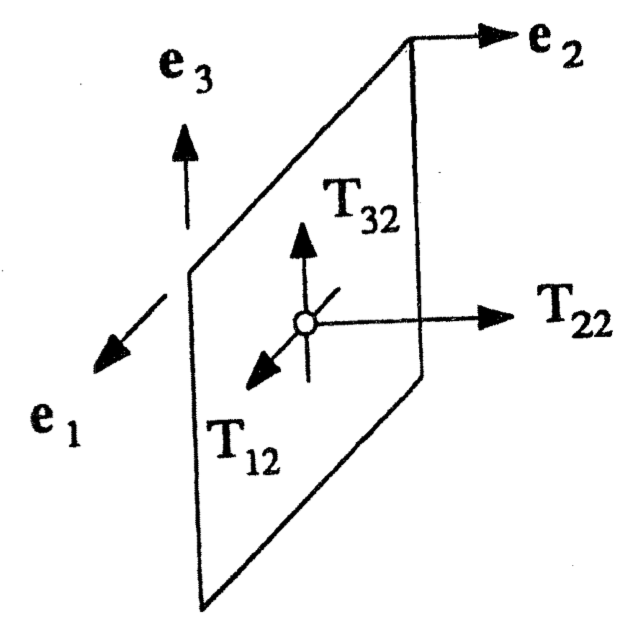
Sign convention for coordinate stresses A positive coordinate stress acts in the direction of the positive coordinate axis on that side of the surface facing the positive direction of a coordinate axis (see Figure 6).
Positive and negative normal stresses are denoted tensile stresses and compressive stresses, respectively.
A variety of symbols for coordinate stresses may be found in other texts: $$ \begin{equation} T_{ik} = \sigma_{ik} = \tau_{ik} \tag{2.59} \end{equation} $$
Additionally, when xyz-coordinates are used, common ways of referring to normall stresses are, \( \sigma_x \) or \( \sigma_{xx} \) etc., and the shear stresses by \( \tau_{xy} \) or \( \sigma_{xy} \). Thus, equivalent representations of the stress matrix \( T \) are: $$ \begin{equation} T = \left [ \begin{array}{ccc} T_{11} & T_{12} & T_{13} \\ T_{21} & T_{22} & T_{23} \\ T_{31} & T_{32} & T_{33} \end{array} \right ] \equiv \left [ \begin{array}{ccc} \sigma_x & \tau_{xy} & \tau_{xz} \\ \tau_{yx} & \sigma_y & \tau_{yz} \\ \tau_{zx} & \tau_{zy} & \sigma_z \end{array} \right ] \equiv \left [ \begin{array}{ccc} \sigma_{xx} & \tau_{xy} & \tau_{xz} \\ \tau_{yx} & \sigma_{yy} & \tau_{yz} \\ \tau_{zx} & \tau_{zy} & \sigma_{zz} \end{array} \right ] \tag{2.60} \end{equation} $$
In other orthogonal coordinate systems like cylindrical \( (r,\theta,z) \) and spherical \( (r,\theta,\phi) \), the stress matrix have a natural representation: $$ \begin{equation} T= \left [ \begin{array}{ccc} \sigma_r & \tau_{r\theta} & \tau_{rz} \\ \tau_{\theta r} & \sigma_\theta & \tau_{\theta z} \\ \tau_{zr} & \tau_{z\theta} & \sigma_z \end{array} \right ], \qquad T= \left [ \begin{array}{ccc} \sigma_r & \tau_{r\theta} & \tau_{r\phi} \\ \tau_{\theta r} & \sigma_\theta & \tau_{\theta \phi} \\ \tau_{\phi r} & \tau_{\phi\theta} & \sigma_\phi \end{array} \right ] \tag{2.61} \end{equation} $$
Below, some examples are presented to familiarize the reader with the stress concept and coordinate stresses.
2.3.2 Example 1: Uniaxial state of stress
Consider at straight rod with cross-sectional area \( A \), subjected to an axial force \( N \) and orient an orthogonal coordinate system with the \( x_1 \)-axis along the direction of the axial force. The corresponding state of stress for the rod is given by the stress matrix: $$ \begin{equation} T= \left [ \begin{array}{ccc} \sigma & 0 & 0 \\ 0 & 0 & 0 \\ 0 & 0 & 0 \end{array} \right ] , \qquad \sigma = \frac{N}{A} \tag{2.62} \end{equation} $$ The cross-section \( A \) is the subjected to a normal stress \( \sigma \). The cross-section is free of shear, i.e., \( T_{12}=T_{13}=0 \), and sections parallell to the axis of the rod are stress free, \ie \( T_{2i}=T_{3i}= 0 \), with \( i=1\ldots 3 \). Such a state of stress is denoted a uniaxial state of stress.
2.3.3 Example 2: Pure shear stress state
y
Figure 7: Torsion of thin-walled cylinder.
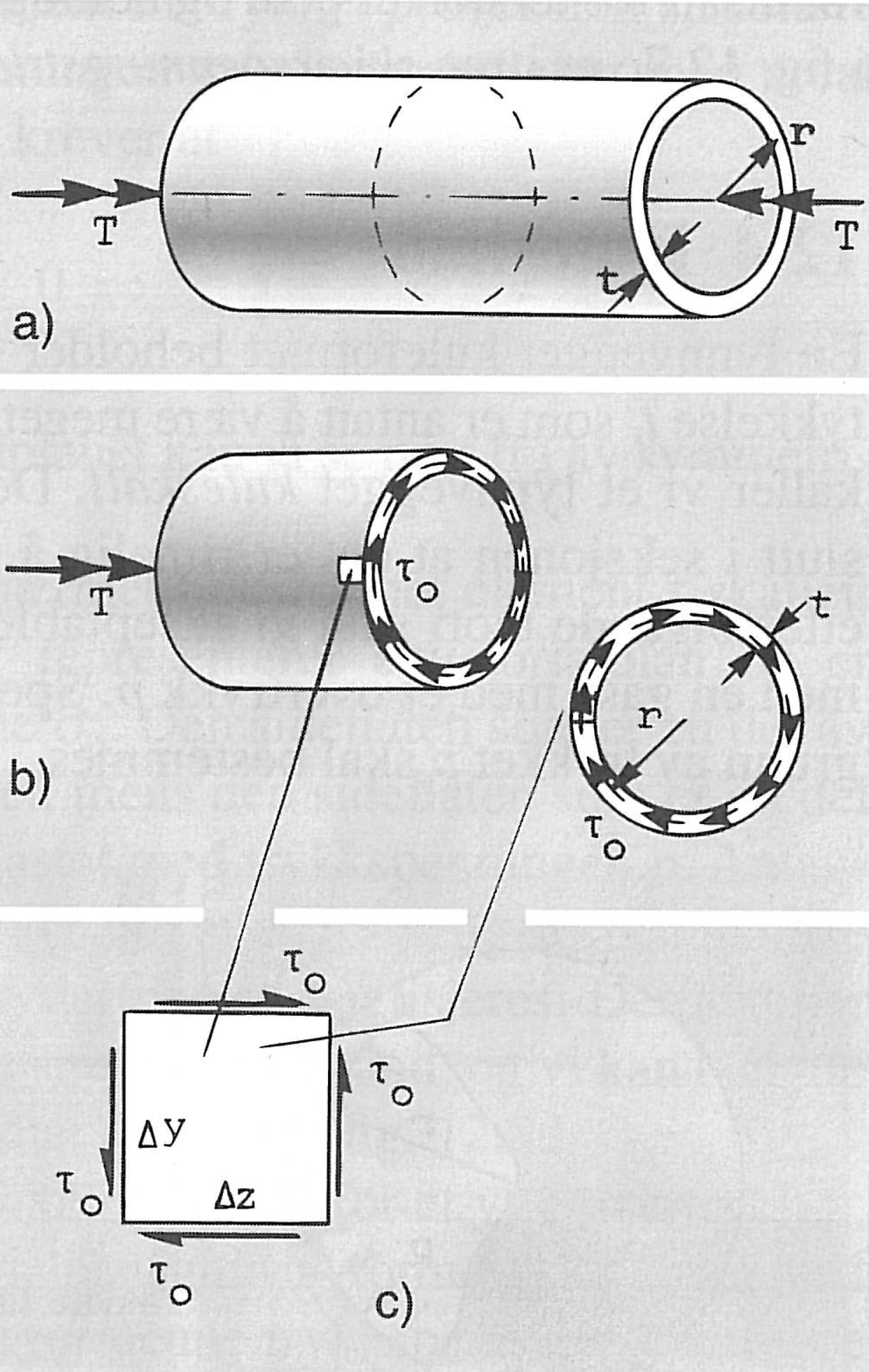
A thin-walled (i.e., \( t\ll r \)) cylinder with mean radius \( r \) and wall thickness \( t \) is subjected to a torsion moment, or torque, \( T \) (see Figure 7). A tangential shear stress \( \tau_0 = \tau_{z\theta} \) constitutes a moment \( \tau_0 \, r \), with respect to the cylinder axis. This is the moment per cross-sectional area, and a first order approximation to the cylindrical cross-sectional area is \( A=2\pi r t \). The moment must balance the imposed torque, and thus we find an expression for the shear stress in the cylinder wall: $$ \begin{equation} \tau_0 = \tau_{z \theta} = \frac{T}{2\pi r^2 t} \tag{2.63} \end{equation} $$ In Figure 7 c) the state of stress in an element of the tube wall is illustrated. We have already found \( \tau_{z\theta} \) and may argue the two force couples must balance for the element to be in equilibrium, and thus: \( \tau_{\theta z} = \tau_{z \theta} = \tau_0 \). We might also have argued that the stress matrix is symmetric, which in fact is based on momentum balance. Thus, the state of state in a wall element of the cylinder may be expressed by: $$ \begin{equation} T= \left [ \begin{array}{ccc} 0 & 0 & 0 \\ 0 & 0 & \tau_0 \\ 0 & \tau_0 & 0 \end{array} \right ] , \qquad \tau_0 = \frac{T}{2\pi r^2 t} \tag{2.64} \end{equation} $$
2.3.4 Cauchy's stress theorem and the Cauchy stress tensor
An important theorem, the Cauchy's stress theorem (CST), will prove useful in the derivation of Cauchy's equations of motion in the section 2.4 Cauchy's equations of motion and the derivation of principal stresses in the section 2.5.1 Principal stresses:
Proof. Consider a tetrahedron as illustrated in Figure 8, with a surface made up of triangles (such a tetrahedron is often referred to as a Cauchy tetrahedron). Three of these triangles are parallell to the orthogonal coordinate planes, intersect the point \( P \) and have areas \( A_k \). The orientation of the fourth triangular plane with surface \( A \), is given by its normal vector \( \mathbf{n} \) and has a distane \( h \) from the point \( P \).
Figure 8: Cauchy's tetrahedron with forces
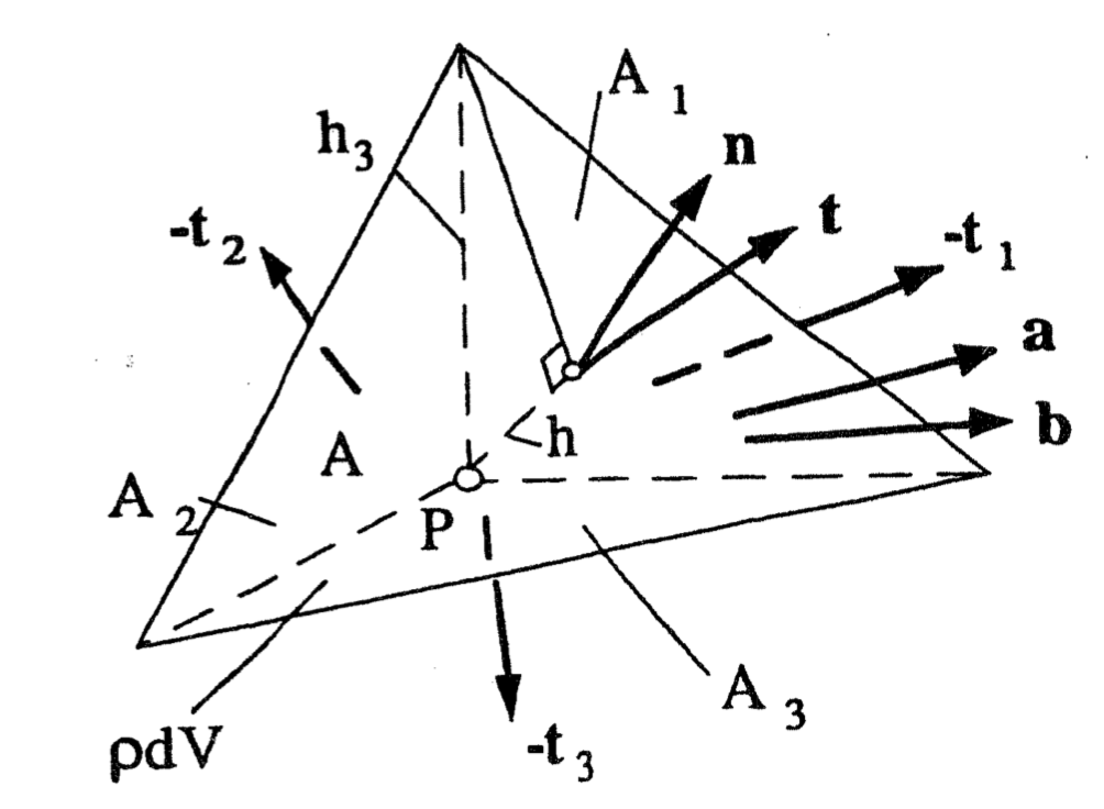
The tetrahedron is subjected to a body force \( \mathbf{b} \), the stress vectors \( -\mathbf{t}_k \) on the coordinate planes, and the stress vector \( \mathbf{t} \) on the last triangle. By claiming balance of linear momentum from (2.44) we get for this tetrahedron: $$ \begin{equation} \sum_{k=1}^3 \int_{A_k} - \mathbf{t}_k \, dA + \int_A \mathbf{t} \, dA + \int_V \mathbf{b} \rho \, dV = \int_V \mathbf{a} \rho \, dV \tag{2.66} \end{equation} $$ If we let \( \mathbf{t}_k \), \( \mathbf{t} \), \( \mathbf{b}\rho \) and \( \mathbf{a} \rho \) represent mean values on the surfaces and in the volume, the equation of motion in (2.66) simplifies to: $$ \begin{equation} -\mathbf{t}_k A_k + \mathbf{t} A + \mathbf{b} \rho V = \mathbf{a} \rho V \tag{2.67} \end{equation} $$
Further, let \( h_k \) denote edges parallel to the base vectors \( \mathbf{e}_k \), and since \( \mathbf{n} \) is a unit vector: $$ \begin{equation} n_k=\frac{h}{h_k} \tag{2.68} \end{equation} $$ To see this, consider the vector \( \boldsymbol{s}_{21} \) from the end of \( h_2 \) to \( h_1 \) which has the components: $$ \begin{equation} \boldsymbol{s}_{21} = (h_1,-h_2,0) \tag{2.69} \end{equation} $$ and correspondingly the vector \( \boldsymbol{s}_{23} \) from the end of \( h_2 \) to \( h_3 \) with components: $$ \begin{equation} \boldsymbol{s}_{23} = (0,-h_2,h_3 ) \tag{2.70} \end{equation} $$
The area \( A \) is then given by the absolute value of the cross-product: $$ \begin{equation} A = | \boldsymbol{s}_{21} \times \boldsymbol{s}_{23} |= \frac{1}{2}\,\sqrt {{h_{{2}}}^{2}{h_{{3}}}^{2}+{h_{{1}}}^{2}{h_{{3}}}^{2}+{h_{ {1}}}^{2}{h_{{2}}}^{2}} \tag{2.71} \end{equation} $$ The volume V may be expressed in four different ways: $$ \begin{equation} V = \frac{1}{3} A h = \frac{1}{3} A_1 h_1 = \frac{1}{3} A_2 h_2 = \frac{1}{3} A_3 h_3 , \quad \text{or} \quad V=\frac{1}{3} A_k h_k \quad \text{no summation} \tag{2.72} \end{equation} $$ and as e.g., \( A_3 = h_2 h_3/2 \) the volume may be expressed by the edges only as: $$ \begin{equation} V = \frac{1}{6}\,h_{{1}}h_{{2}}h_{{3}} \tag{2.73} \end{equation} $$ By combination of equations (2.71), (3.32), and (2.73) we get an expression for \( h \): $$ \begin{equation} h= \frac {h_{{1}}h_{{2}}h_{{3}}}{\sqrt {{h_{{2}}}^{2}{h_{{3}}}^{2}+{h_{{ 1}}}^{2}{h_{{3}}}^{2}+{h_{{1}}}^{2}{h_{{2}}}^{2}}} = \frac {h_{{1}}h_{{2}}h_{{3}}}{2 \, A} \tag{2.74} \end{equation} $$ An expression for a unit normal vector to \( A \) may be found by: $$ \begin{equation} \boldsymbol{n} = \pm \frac{\boldsymbol{s}_{21} \times \boldsymbol{s}_{23}}{| \boldsymbol{s}_{21} \times \boldsymbol{s}_{23} |} = \pm \frac{\boldsymbol{s}_{21} \times \boldsymbol{s}_{23}}{2 \, A} \tag{2.75} \end{equation} $$ we choose the version with positive components for convenience: $$ \begin{equation} \boldsymbol{n} = \frac{(h_{{2}}h_{{3}}, h_{{1}} h_{{3}}, h_{{1}}h_{{2}})}{2A} = h \left (\frac{1}{h_1}, \frac{1}{h_2} ,\frac{1}{h_3}\right) \tag{2.76} \end{equation} $$ where the latter equality of equation (2.76) follows from equation (2.74). Thus, we have derived a convenient expression for the normal vector, which is given on component for in equation (2.68).
By combination of (2.68) and (2.72) we get: $$ \begin{equation} A_k = A n_k \quad \mathrm{and} \qquad V = \frac{1}{3} A h \tag{2.77} \end{equation} $$ And subsequently, by substitution of the geometric relations in (2.77) into (2.67) we obtain: $$ \begin{equation} -\mathbf{t}_k n_k + \mathbf{t} + \mathbf{b} \rho \frac{h}{3} = \mathbf{a} \rho \frac{h}{3} \tag{2.78} \end{equation} $$ By letting \( h \rightarrow 0 \) in (2.78), the only terms left are the ones pertaining to surface stresses, which yields: $$ \begin{equation} \mathbf{t} = \mathbf{t}_k n_k \tag{2.79} \end{equation} $$ From the definition of coordinate stresses ((2.57)) we have \( \mathbf{t}_k = T_{ik} \mathbf{e}_i \) which by substitution into (2.79) yields $$ \begin{equation} \mathbf{t} = T_{ik} n_k \mathbf{e}_i \Leftrightarrow t_i = T_{ik} n_k \tag{2.80} \end{equation} $$ and thus completes the proof of Cauchy's stress theorem.
The CST express how the coordinate stresses \( T_{ik} \) completely determines the state of stress in a particle. Both the stress vector \( \mathbf{t} \) and the unit normal \( \mathbf{n} \) are coordinate invariant particle properties(i.e., independent of choice of coordinate system), which implies that (2.65) has a coordinate invariant character. In this presentation we simply state that the stress vector \( \mathbf{t} \) may be expressed by the vector \( \mathbf{n} \), by an operator \( \mathbf{T} \). We denote this operator the stress tensor \( \mathbf{T} \), which in a given coordinate system Ox is represented by the matrix \( T \). The stress tensor \( \mathbf{T} \) is a coordinate invariant, intensive quantity that in any Cartesian coordinate system is represented by the corresponding stress matrix \( T \) (in the same manner as for vectors). The coordinate stresses \( T_{ik} \) are the components of the stress tensor in a particular coordinate system.
Figure 9: Decomposition of the stress vector \( \mathbf{t} \).
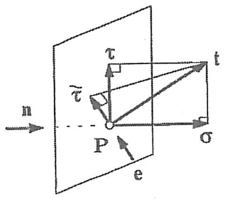
Based on the CST, we may now find expressions for the normal stress component and the shear stress component of the stress vector \( \mathbf{t} \). The normal stress \( \sigma \), is the component of \( \mathbf{t} \), acting in the direction of the surface normal \( \mathbf{n} \), and is thus found by the scalar product between the two vectors: $$ \begin{equation} \sigma = \mathbf{n \cdot t} = \mathbf{n \cdot T \cdot n} = n_i T_{ik} n_k \tag{2.81} \end{equation} $$
The component of \( \mathbf{t} \), remaining after subtraction of the normal stress, is denoted the shear stress vector \( \boldsymbol{\tau} \) and is orthogonal to \( \mathbf{n} \) and aligned with the surface: $$ \begin{equation} \boldsymbol{\tau} = \mathbf{t} - \sigma \mathbf{n}, \qquad \boldsymbol{\tau} \cdot \mathbf{n} = 0 \tag{2.82} \end{equation} $$
The magnitude of the shear stress vector is simply denoted shear stress \( \tau \), and may be expressed: $$ \begin{equation} \tau =\sqrt{\tau_i\tau_i} = \sqrt{t_i^2 - 2 \sigma t_i n_i + \sigma^2 n_i^2} = \sqrt{\mathbf{t}\cdot\mathbf{t} - \sigma^2} \tag{2.83} \end{equation} $$ by the use of (2.81).
Further, the component $\tau_e$of the stress vector \( \mathbf{t} \) acting on the surface with orientation \( \mathbf{n} \), in an arbitrary direction \( \mathbf{e} \) by: $$ \begin{equation} \tau_e = \mathbf{e} \cdot \mathbf{t}= \mathbf{e \cdot T \cdot n} = e_i T_{ik} n_k \tag{2.84} \end{equation} $$ By selecting \( \mathbf{e} \) and \( \mathbf{n} \) as the base vectors \( \mathbf{e}_i \) and \( \mathbf{e}_k \), respectively, in a general Cartesian coordinate system Ox, the coordinate stresses (or components) of the stress tensor \( \mathbf{T} \) may be expressed as: $$ \begin{equation} T_{ik} = \mathbf{e}_i \cdot \mathbf{T} \cdot \mathbf{e}_k \tag{2.85} \end{equation} $$
2.3.5 Example 3: Example: Fluid at rest: Isotropic state of stress
In the section 5.1 Introduction we define a fluid as a material that deforms continuously when subjected to an anisotropic state of stress. Conversely, no deformation implies an isotropic state of stress, i.e., all material surfaces through a fluid particle transmits the same normal stress. This normal stress is what conventionally is denoted the pressure \( p \), and the shear stresses on the surfaces are zero. The stress matrix in any Cartesian coordinate system Ox is therefore for a fluid at rest: $$ \begin{equation} \mathbf{T} = \left [ \begin{array}{ccc} -p & 0 & 0 \\ 0 & -p & 0 \\ 0 & 0 & -p \end{array} \right ] = -p \mathbf{I} \tag{2.86} \end{equation} $$