3.3 Small strains and small deformations
For a wide range of loading conditions on typical structural materials (e.g., steel, aluminum, concrete, wood) the resulting strains are small. A state for which the absolute value of the longitudinal strains are less than \( 1\% \), will be referred to as a state of small strains . In biomechanical applications however, small strains are the exception rather than the rule. Still, an exposition of the strain measures subject to the state of small strain is provided below, as they are simpler and thus more understandable than their large strain counterparts.
3.3.1 Small strains
Figure 19: Illustrations of small strains and large deformations.
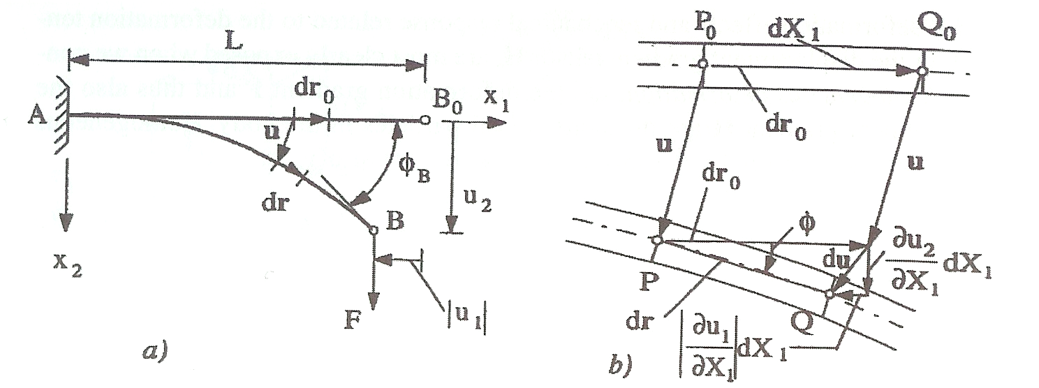
Note that small strains do not necessarily imply that either displacements or rotations of a line element are small (see Figure 19 adapted from fig 5.3.1 in cite[]{irgens08}).
Longitudinal strain We assume a state of small strains, i.e., \( \epsilon < 1\% \). Then the generic expression for \( \epsilon \) in (3.17) may be reformulated: $$ \begin{equation} \left( {1 + \epsilon } \right)^2 = 1 + 2\epsilon + \epsilon ^2 = \boldsymbol{n \cdot C \cdot n} = \boldsymbol{1} + 2\;\boldsymbol{n} \cdot \boldsymbol{E} \cdot \boldsymbol{n} \tag{3.37} \end{equation} $$ From (3.37) an expression for \( \epsilon \) valid for small strains is obtained by dropping higher order terms in \( \epsilon \) $$ \begin{equation} \epsilon = \boldsymbol{n} \cdot \boldsymbol{E} \cdot \boldsymbol{n} = n_i E_{ij} n_j \tag{3.38} \end{equation} $$
Similarly, an expression for the shear strain for small strains is obtained from (3.30), by setting \( \gamma \approx \sin \gamma \) and the denominator to 1: $$ \begin{equation} \gamma = 2\;\bar{\boldsymbol{n}} \cdot \boldsymbol{E} \cdot \boldsymbol{n} = 2\;\bar n_i E_{ij} n_j = \bar{\boldsymbol{n}} \cdot \boldsymbol{C} \cdot \boldsymbol{n} = \bar n_i C_{ij} n_j \tag{3.39} \end{equation} $$ Coordinate strains may then naturally be introduced whenever material line elements in \( K_0 \) are parallel to the reference coordinate system: $$ \begin{equation} \epsilon_{ii} = E_{ii} \quad \text{no summation}, \quad \gamma_{ij} = 2\, E_{ij} \quad i \neq j \tag{3.40} \end{equation} $$ Further, rearrangement of (3.36) for the volumetric strain \( \epsilon_v \) yields: $$ \begin{align} 1 + 2\epsilon _v + \epsilon _v^2 = \det ({\boldsymbol{1}} + 2{\boldsymbol{E}}) = 1 + 2\, E_{kk} + \mathcal{O}(E_{ik}\,E_{lm}) \tag{3.41} \end{align} $$ which by neglection of higher order terms (i.e., \( \epsilon _v^2 \) and \( \mathcal{O}(E_{ik}\,E_{lm}) \)) yields and expression for the volumetric strain \( \epsilon_v \) valid for small strains: $$ \begin{equation} \epsilon _v = \tr(\boldsymbol{E}) \tag{3.42} \end{equation} $$
3.3.2 Small deformations
To relate the concept of small deformations to the elements in the displacement gradient tensor \( \mathbf{H} \), consider the deformation of a line element \( PQ \) along the beam \( AB \) in Figure 19 a), where \( P_0Q_0 \) denote \( PQ \) in the reference configuration or in the undeformed case (Figure 19 b)). Small deformations will conventionally imply both a small angle of rotation \( \phi \), and small strain, which from Figure 19 b), is seen to be satisfied when: $$ \begin{equation} \tag{3.43} \left |\partd{u_2}{X_1} \right | \equiv |H_{21}| \ll 1 \qquad\text{ and } \qquad \left |\partd{u_1}{X_1} \right | \equiv |H_{11}| \ll 1 \end{equation} $$
Small deformations In the general case, the condition of small deformations is defined by the requirement that all components of the displacement gradient tensor \( H_{ik} \) must be small $$ \begin{equation} \tag{3.44} \left| {H_{ij} } \right| = \left| {\frac{{\partial u_i }}{{\partial X_j }}} \right| \ll 1\quad \Leftrightarrow \quad norm\left( {\boldsymbol{H}} \right) \ll 1 \end{equation} $$
Small deformations imply both small strains and small rotations. Occasionally infinitesimal deformations is used as a synonym in the literature for small deformations.
Now, the assumption of small deformations has implications for how one may interpret gradients and derivatives. For example for an arbitrary field \( f(\mathbf{r},t) = f(\mathbf{r}(\mathbf{r}_0,t),t) \), one may obtain by using Eq. (3.18) $$ \begin{equation} \tag{3.45} \frac{{\partial f}}{{\partial X_j }} = \frac{{\partial f}}{{\partial x_k }}\frac{{\partial x_k }}{{\partial X_j }} = \frac{{\partial f}}{{\partial x_k }}\left( {\delta _{ki} + \frac{{\partial u_k }}{{\partial X_i }}} \right) \approx \partd{f}{x_i} \equiv f_{,i} \end{equation} $$ which means that the spatial gradient in the current and in the reference configuration are the same.
Normally, small deformations imply small displacements, and we may replace the particle reference \( \mathbf{r}_0 \) by the position vector \( \mathbf{r} \), and consequently use the position coordinates \( x_i \) as particle coordinates, rather than \( X_i \). For the same reason we will also have for small displacements/deformations: $$ \begin{equation} \tag{3.46} \dot{f}(\mathbf{r},t) = \dot{f}(x,t) = \partial_t f (\mathbf{r},t) \equiv \partd{f(\mathbf{r},t)}{t} \end{equation} $$ which means that the particle derivative and the partial derivative with respect to time are equivalent subject to the small displacements assumption.
Further, the displacement gradient are also simplified for small displacements (compare Eq. (3.19) ): $$ \begin{equation} \tag{3.47} H_{ij} = u_{i,j} \qquad \Leftrightarrow \qquad \mathbf{H} = *grad* \mathbf{u} \end{equation} $$ and the Green strain tensor Equation (3.23) reduce to: $$ \begin{equation} \tag{3.48} {\bf{E}} = \frac{1}{2}\left( {{\bf{H + H}}^T } \right)\quad \Leftrightarrow \quad E_{ij} = \frac{1}{2}\left( {u_{i,j} + u_{j,i} } \right) \end{equation} $$
From Eq. (3.48) we may infer that the expressions for the coordinate strains reduce to: $$ \begin{equation} \tag{3.49} \epsilon_{11} = E_{11} = u_{1,1}, \qquad \gamma_{12} = 2E_{12} = u_{1,2} + u_{2,1}, \qquad \text{etc.} \end{equation} $$
Figure 20: Two-dimensional illustration of coordinate strains.
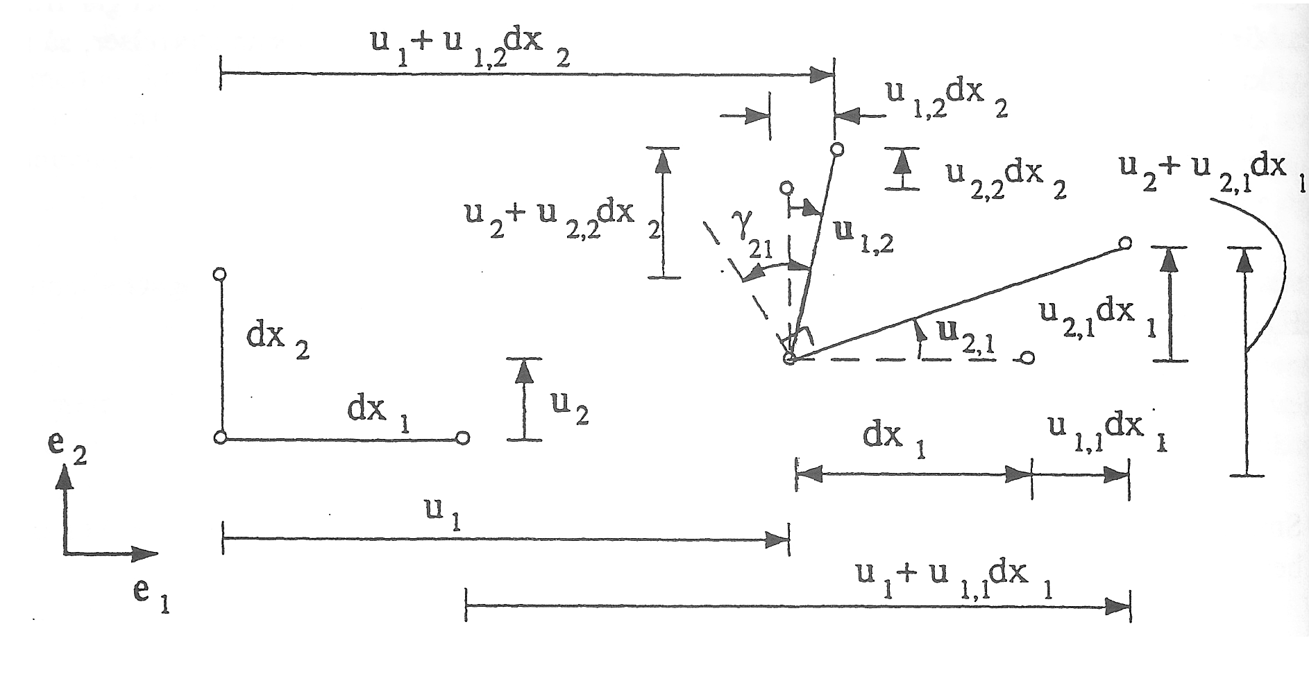
The expressions for coordinate strains in Eq. (3.49) are illustrated in Figure 20 in the two-dimensional case.
As for small strains the volumetric strain \( \epsilon_v \) for small displacements reduces to: $$ \begin{equation} \epsilon_{v} = \tr \mathbf{E} =E_{kk} = u_{k,k} = \div \mathbf{u} \tag{3.50} \end{equation} $$ From Eq. (3.50) we realize that the divergence of the displacement vector is an expression for the change of volume per unit volume, when the material in question has been transformed from the undeformed reference configuration \( K_0 \) to the deformed current configuration \( K \).
3.3.3 Principal strains
In the section 3.3.1 Small strains expressions were derived for longitudinal strain \( \epsilon \) and shear strain \( \gamma \) (see (3.38) and (3.39)), valid for states of small strain: $$ \begin{equation} \epsilon = \boldsymbol{n} \cdot \boldsymbol{E} \cdot \boldsymbol{n} = n_i E_{ij} n_j, \quad % \gamma = 2\, \bar{\boldsymbol{n}} \cdot \boldsymbol{E} \cdot \boldsymbol{n} = 2\, \bar{n}_i E_{ij} n_j \tag{3.51} \end{equation} $$ As the Green strain tensor is symmetric by construction (see (3.23)), three orthogonal principal strain directions with corresponding principal strain values may be found. % \index{Principal strain direction} % This result is the strain equivalent to the principal stress theorem (2.114). However, we do not have a Cauchy stress theorem (2.65) equivalent for strains, as no vector for strains have been introduced. Rather, for any direction \( \boldsymbol{n} \) in \( K_0 \) we define a vector \( \boldsymbol{E \cdot n} \). The longitudinal strain in the direction of \( \boldsymbol{n} \) is then the projection of the vector \( \boldsymbol{E \cdot n} \) in the direction of \( \boldsymbol{n} \): $$ \begin{equation} \epsilon = \boldsymbol{n} \cdot (\boldsymbol{E} \cdot \boldsymbol{n}) = n_i E_{ij} n_j, \quad % \tag{3.52} \end{equation} $$ Similarly, the shear strain is equal to twice the component of \( \boldsymbol{E \cdot n} \) in the direction of \( \bar{\boldsymbol{n}} \): $$ \begin{equation} \gamma = 2\, \bar{\boldsymbol{n}} \cdot (\boldsymbol{E} \cdot \boldsymbol{n}) = 2\, \bar{n}_i E_{ij} n_j \tag{3.53} \end{equation} $$ The conditions for the principal strains \( \epsilon_i \) and the corresponding principal directions \( \boldsymbol{n}_i \) forms an eigenvalue problem : $$ \begin{equation} \boldsymbol{E \cdot n} = \epsilon \boldsymbol{n} \Leftrightarrow % \left (\epsilon \boldsymbol{1 - E} \right ) \cdot \boldsymbol{n} = 0 \Leftrightarrow % \left (\epsilon \delta_{ij} - E_{ij} \right ) n_{j} = 0 \tag{3.54} \end{equation} $$ with corresponding characteristic equation for the small strain tensor \( \boldsymbol{E} \): $$ \begin{equation} \epsilon^3 - I \epsilon^2 + I\!I \epsilon - I\!I\!I = 0 \tag{3.55} \end{equation} $$ and where the principal invariants \( I \), \( I\!I \), and \( I\!I\!I \) of the strain tensor \( \boldsymbol{E} \) are given by: $$ \begin{align} I &= \tr\boldsymbol{E} = E_{kk} \tag{3.56}\\ I\!I &= \frac{1}{2} \left [ (\tr\boldsymbol{E})^2 - \|\boldsymbol{E}\|^2 \right ] = % \frac{1}{2} \left [ E_{ii}E_{jj} - E_{ij} E_{ij} \right ] \tag{3.57}\\ I\!I\!I & = \det \boldsymbol{E} = e_{ijk} E_{i1} E_{j2} E_{k3} \tag{3.58} \end{align} $$ The characteristic equation (3.55) has three real solutions, the principal strains \( \epsilon_i \). Their corresponding principal directions \( \boldsymbol{n}_i \) are orthogonal, subject to the condition that all principal strains are different. In general three orthogonal directions may always be specified. From (3.54) and (3.53), the shear strains related to principal directions are seen to be zero. From the above we formulate the following theorem:
The principal strains in a particle represent extremal values of longitudinal strains. By ordering the longitudinal strains such that: \( \epsilon_3 < \epsilon_2 < \epsilon_1 \), we get: $$ \begin{equation} \epsilon_{\max} = \epsilon_1, \quad \epsilon_{\min} = \epsilon_3 \tag{3.59} \end{equation} $$ Further, the maximum shear strain is given by: $$ \begin{equation} \gamma_{\max} = \epsilon_{\max} -\epsilon_{\min} \tag{3.60} \end{equation} $$ for the directions: $$ \begin{equation} \boldsymbol{n} = \frac{\boldsymbol{n}_1 + \boldsymbol{n}_3}{\sqrt{2}}, \quad % \bar{\boldsymbol{n}} = \frac{\boldsymbol{n}_1 - \boldsymbol{n}_3}{\sqrt{2}} \tag{3.61} \end{equation} $$
3.3.4 Small strains in a surface
Measurements of strains or deformation are generally easier to perform, than measurements of stresses or forces. Additionally, given an appropriate material model, stresses may be derived for measured strains. Strain measurements are often performed by using strain rosettes. In the following we shall analyze the state of strain in a surface in a surface and introduce a coordinate system with its \( x_3 \)-axis normal to the tangent plane of the surface.
Figure 21: Orthogonal unit vectors \( \mathbf{n} \) and \( \bar{\mathbf{n}} \) in a material surface.

The two other axes will then be tangent plane to the surface in which the strains are located. Two orthogonal unit vectors in the tangent plane \( \boldsymbol{n} \) and \( \bar{\boldsymbol{n}} \) may then be expressed by their angle with respect to \( x_1 \)-axis (see Fig. 21). $$ \begin{equation} \boldsymbol{n} = [\cos \phi, \sin \phi, 0], \quad \bar{\boldsymbol{n}} = [\sin \phi, -\cos \phi, 0] \tag{3.62} \end{equation} $$
The longitudinal strain in the \( \boldsymbol{n} \)-direction and the shear strain with respect to \( \boldsymbol{n} \) and \( \bar{\boldsymbol{n}} \) is given by (3.38) and (3.39): $$ \begin{align} \epsilon & = \epsilon(\phi) = \boldsymbol{n \cdot E \cdot n} = n_{\alpha} E_{\alpha\beta} n_{\beta} = E_{11} \cos^2 \phi + E_{22} \sin^2 \phi + 2 E_{12} \cos \phi \sin \phi \tag{3.63}\\ \gamma &= \gamma(\phi) = 2 \, \boldsymbol{\bar{n} \cdot E \cdot n} = 2 \bar{n}_\alpha E_{\alpha\beta} n_\beta \notag \tag{3.64}\\ & = 2 \left [ E_{11} \sin \phi \cos \phi - E_{22} \cos \phi \sin \phi - E_{12} (\cos^2 \phi - \sin^2 \phi) \right ] \tag{3.65} \end{align} $$
The conventional notation for coordinate strains is then introduced: $$ \begin{equation} \epsilon_x = E_{11}, \quad \epsilon_y = E_{22}, \quad \gamma_{xy} = 2 E_{12} \tag{3.66} \end{equation} $$ Then, by employing the trigonometric formulas for \( \sin 2\phi \) and \( \cos 2 \phi \) in (8.2)) and (3.66), the expressions for strains in (3.63) and (3.65) may be transformed to: $$ \begin{align} \epsilon(\phi) &= \frac{\epsilon_x + \epsilon_y}{2} + \frac{\epsilon_x - \epsilon_y}{2} \, \cos 2 \phi + \frac{1}{2} \sin 2\phi \tag{3.67}\\ \gamma(\phi) &= (\epsilon_x + \epsilon_y) \sin 2 \phi - \gamma_{xy} \cos 2 \phi \tag{3.68} \end{align} $$ These formulas are equivalent to those derived for plane stress in the section 2.5.3 Planar stress, and the formulas for principal strains in the surface \( \epsilon_1 \) and \( \epsilon_2 \), and the angle \( \phi_1 \) for the principle direction, follow directly from the corresponding formulas for plane stress (see Eqs. (2.159) and (2.160)): $$ \begin{align} \epsilon_{1,2}& = \frac{\epsilon_x + \epsilon_y}{2} \pm % \sqrt{\left ( \frac{\epsilon_x - \epsilon_y}{2} \right )^2 + \left (\frac{\gamma_{xy}}{2} \right )^2} \tag{3.69}\\ \phi_1 & = \arctan 2 \frac{\epsilon_x - \epsilon_y}{\gamma_{xy}} \tag{3.70} \end{align} $$ Note that the \( x_3 \)-direction need not necessarily be a principal direction, and consequently the expressions in (3.69) are not necessarily principal strains for the general state of strain. However, this will be the case in many situations, e.g., for a thin-walled isotropic geometry.
Similarly, the expression for the maximum shear strain in the surface are equivalent to the shear stress expressions (Eq. (2.161)), and may be presented: $$ \begin{equation} \gamma_{\max} = |\epsilon_1 - \epsilon_2 | = 2\, \sqrt{\left ( \frac{\epsilon_x - \epsilon_y}{2} \right )^2 + \left (\frac{\gamma_{xy}}{2} \right )^2} \tag{3.71} \end{equation} $$ Thus, from Eq. (3.71) we see that \( \gamma_{\max} \) may be computed either form the principal strains or from the coordinate strains.
3.3.5 Example 7: Strain rosettes
Figure 22: \( 0^{\circ}-45^{\circ}-90^{\circ} \) rectangular strain rosette.

As previously stated in the beginning of the section 3.3.4 Small strains in a surface, measurements of strains or deformation are generally easier to perform, than measurements of stresses or forces. In this example we show the principal strains may be calculated based on measurements from a \( 0^{\circ} \)-$45^{\circ}$-\( 90^{\circ} \) rectangular strain rosette (Figure 22).
Note that if the material in question is well characterized, one may deduce the principal stresses from the principal strains.
From the previous expressions for small strains in a surface (3.67) and (3.68) we have: $$ \begin{equation} \epsilon_{45} \equiv \epsilon (\phi=45^\circ) = \frac{\epsilon_x + \epsilon_y}{2} + \frac{1}{2} \, \gamma_{xy} \quad \Rightarrow \quad \gamma_{xy} = 2 \epsilon_{45} - \epsilon_x - \epsilon_y \tag{3.72} \end{equation} $$ Note that (3.67) and (3.68) also yield \( \epsilon_0 \equiv \epsilon(\phi=0)= \epsilon_x \) and \( \epsilon_{90} \equiv \epsilon(\phi=90^\circ)= \epsilon_y \). With the expression for \( \gamma_{xy} \) at hand we may readily compute the principal strains by substitution into (3.69): $$ \begin{align} \epsilon_{1,2}& = \frac{\epsilon_x + \epsilon_y}{2} \pm % \sqrt{\frac{1}{2} \, \left ( \epsilon_x^2 + \epsilon_y^2 \right ) % + \epsilon_{45} \left (\epsilon_{45} - \epsilon_x - \epsilon_y \right )} \tag{3.73}\\ \phi_1 & = \arctan \frac{2\, \epsilon_{45} - \epsilon_x- \epsilon_y}{2\,(\epsilon_1 -\epsilon_y)} \tag{3.74} \end{align} $$
Thus, we see that the principal strains \( \epsilon_1 \) and \( \epsilon_2 \) are determined completely by the measurements of \( \epsilon_{45} \), \( \epsilon_x \), \( \epsilon_y \).
1: Indices are dropped for clarity.