7.2 Infinitesimal derivation of the 1D governing equations for a compliant vessel
In this section the 1D governing equations for mass and momentum will be derived in a somewhat simpler way than in section (7.3 Integral derivation of the 1D governing equations for a compliant vessel). In the derivation we will first consider mass and momentum for a control volume. However, the length of the control volume will later be reduced to zero. Thus, higher order terms may be neglected for several terms.
Some of the first scientific papers on this issue include [24] [25] [26].
7.2.1 Conservation of mass
Blood may normally be considered incompressible (\( \rho = \text{constant} \)) and thus conservation of mass per time unit reduces to: $$ \begin{equation} \dot{V} = Q_i - Q_o \tag{7.6} \end{equation} $$ where \( \dot{V} \) denotes rate of change in volume, whereas \( Q_{i} \) and \( Q_o \) is volume flow rate in and out of the volume, respectively (see Figure 68).
Figure 68: A deformable control volume with fixed endpoints.
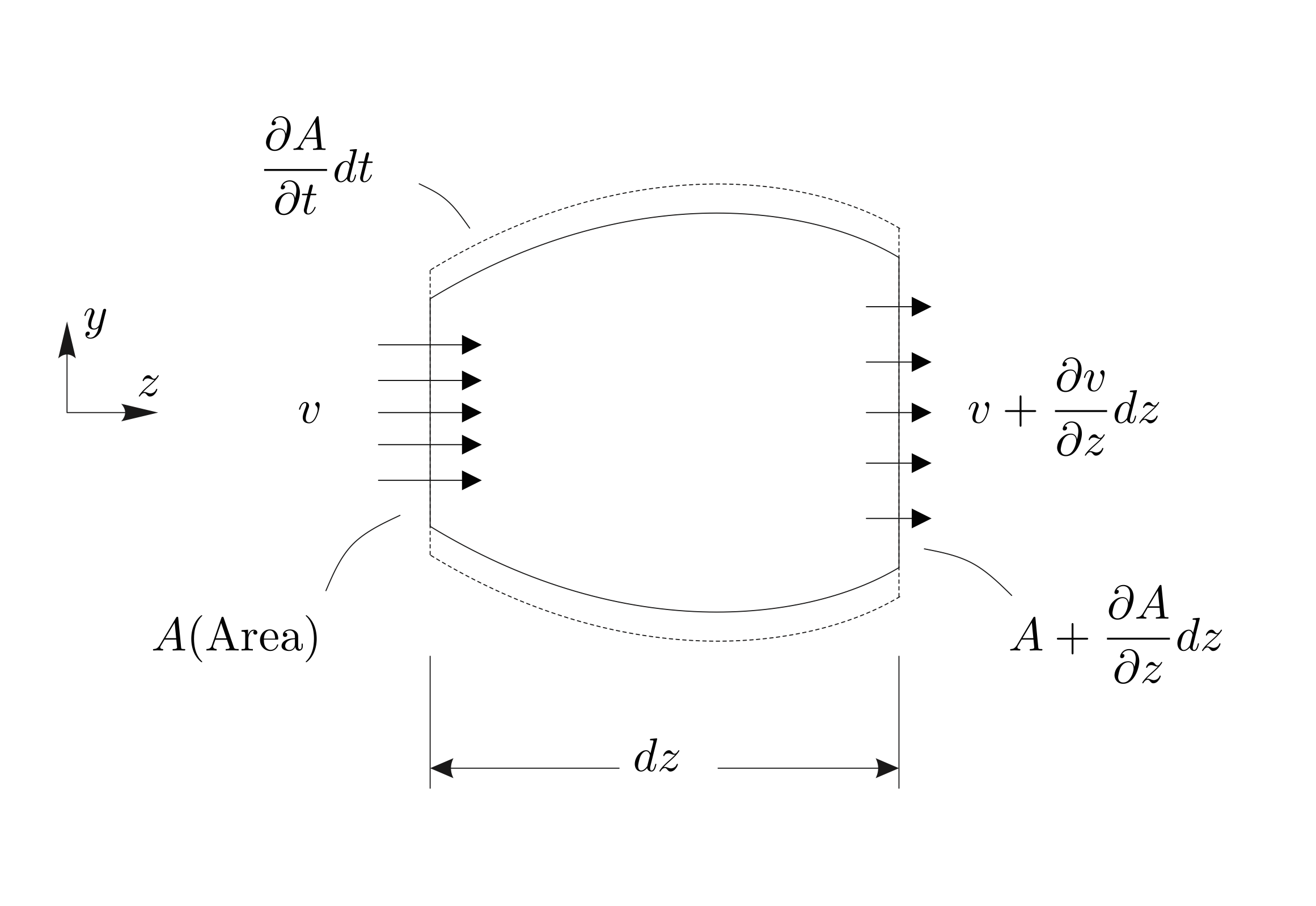
By adopting the convention in ((7.43)) of the section 7.3 Integral derivation of the 1D governing equations for a compliant vessel the volumetric influx into the volume \( Q_i \) (Figure 68) may be expressed by: $$ \begin{equation} Q_{i}=\int_{A_0} v_3 \dA = v A \tag{7.7} \end{equation} $$ For the outflux the spatial changes in the velocity in the axial direction must be accounted for: $$ \begin{equation} Q_{o} =\int_A \left ( v_3 + \partd{v_3}{z} \, dz \right )\, \dA \approx v A + \partd{(vA)}{z} \dz, \quad A_0 = A + \partd{A}{z} \, dz \tag{7.8} \end{equation} $$
The deformation of the volume is assumed to be homogeneous in the axial direction and consequently the rate of change in volume may be expressed by: $$ \begin{equation} \dot{V} \approx \frac{\partial A}{\partial t} \, dz \tag{7.9} \end{equation} $$ Note, that the assumption of homogeneous deformation has no significant bearings as the length \( dz \) control volume collapse to zero in the final expression.
Finally, the equation for conservation of mass is obtained by combination of (7.6), (7.7), (7.8) and (7.9) and subsequent division by \( dz \) : $$ \begin{equation} \partd{A}{t} + \partd{Av}{z} = 0 \tag{7.10} \end{equation} $$
The equation for mass conservation in (7.10) may alternatively be derived by using the Reynolds transport theorem for deformable control volumes (2.33). As for the former derivation in this section, we assume a control volume which deforms with the compliant vessels, but tether the endpoints (see Figure 68). The mass equation is obtained by letting the generic intensive property \( b \) be the mass density \( \rho \): $$ \begin{equation} \tag{7.11} \dot{m} = \frac{d m}{dt} = \ddt \Int_{V_c(t)} \rho \, dV + \Int_{A_c(t)} \rho \, (\boldsymbol{v} -\boldsymbol{v}_c )\cdot \boldsymbol{n} \, dA = 0 \end{equation} $$ Note, that the control volume velocity \( \boldsymbol{v}_c = 0 \) at the fixed endpoints \( z_1 \) and \( z_2 \) of \( V_c(t) \) the control volume, whereas \( \boldsymbol{v}_c=\boldsymbol{v} \) at the compliant vessel wall. Thus, the flux terms in (7.11) will only give contributions at the endpoints, as the flux at the the vessel wall be zero. Further, the time derivative of the volume integral in (7.11) may be put inside the integral sign if the axial coordinate \( z \) is iterated first: $$ \begin{equation} \tag{7.12} \dot{m} = \Int_{z_1}^{z_2} \partd{(\rho A)}{t} \; dz + (\rho v A)_2 - (\rho v A)_1 = 0 \end{equation} $$ where \( v = \bar{v}_z \), i.e., the cross-sectional averaged z-component of \( \boldsymbol{v} \), \( A=A(z) \) is the cross-sectional area at any location \( z \). The subscripts of the flux terms refers to location \( z_1 \) and \( z_2 \), respectively. By assuming a constant density \( \rho \) of the fluid in the compliant vessel, it may be eliminated from (7.12) to yield: $$ \begin{equation} \tag{7.13} \dot{m} = \Int_{z_1}^{z_2} \partd{A}{t} + \partd{v A}{z} \; dz = 0 \end{equation} $$ As (7.13) must be valid for any choice of \( V_c(t) \), i.e., \( z_1 \) and \( z_2 \), the integrand must vanish, and thus the differential form of the mass conservation equation given in (7.10) is obtained. As \( vA=Q \) an equivalent equation for mass conservation is: $$ \begin{equation} \tag{7.14} \partd{A}{t} + \partd{Q}{z} = 0 \end{equation} $$
7.2.2 The momentum equation
Figure 69: Outline of control volume with pressure and velocity.

The derivation of the momentum equation is based on Euler's first axiom which states that the rate of linear momentum is balanced balanced by the net force. In this section we will express the various contributions to the net force and subsequently present an expression for the rate of linear momentum, which will lead us to a momentum equation.
The first force contribution we will consider is that of pressure. As can be seen from Figure 69, pressure will contribute on all surfaces of our control volume. The pressure force acting on the left hand side will be: $$ \begin{equation} \tag{7.15} F_{p_i} = pA \end{equation} $$ On the right hand side the expression for the pressure contribution is somewhat more complicated: $$ \begin{equation} F_{p_o} = - \left (p + \partd{p}{z} \, dz \right ) \left (A + \partd{A}{z} dz \right ) \tag{7.16} \end{equation} $$ The pressure acting on the surface \( A \) will also have an axial contribution which may be shown to be: $$ \begin{equation} \tag{7.17} F_{p_A}= p \partd{A}{z} \, dz \end{equation} $$
Wall friction may be accounted for by introducing the wall shear stress \( \tau \), which will be a function of the cross-wise velocity profile (see (7.71)). In order to derive the momentum equation it will suffice to present the viscous force contribution as: $$ \begin{equation} F_{\tau}=\tau \pi D \, dz \tag{7.18} \end{equation} $$
Finally, the net force is found by summation of (7.15), (7.16), (7.17), and (7.18): $$ \begin{equation} \tag{7.19} F_{\text{net}} = -A \partd{p}{z} \, dz + \tau \pi D \, dz \end{equation} $$
Further, we need an expression for the rate of change of linear momentum \( \boldsymbol{P} \) (see (2.6)) in the z-direction, and employ the Reynolds transport theorem for deformable control volumes, in the same manner as for the derivation of the mass conservation equation. $$ \begin{equation} \tag{7.20} \dot{{P}_z} = \ddt \Int_{V_c(t)} \rho v_z \, dV + \Int_{A_c(t)} \rho v_z\, (\boldsymbol{v} -\boldsymbol{v}_c )\cdot \boldsymbol{n} \, dA \end{equation} $$ which, by arguing in the same manner as for the mass conservation derivation, may be simplified to: $$ \begin{equation} \tag{7.21} \dot{P_z} = \Int_{z_1}^{z_2} \partd{\rho \overline{v_z} A}{t}\, dz + (\rho \overline{v_z^2} A)_2 - (\rho \overline{v_z^2} A)_1 \end{equation} $$ By assuming a flat velocity profile we have \( \overline{v_z^2} = \bar{v}_z^2 \) and by further simplification of the notation by \( v=\bar{v}_z \) we get:
Finally, a momentum equation may be formed by assembling the rate of change of linear momentum in equation (7.21) and the net force in equation (7.19): $$ \begin{equation} \partd{v}{t} + v\partd{v}{z} = - \frac{1}{\rho} \partd{p}{z}+ \frac{\pi D}{\rho A}\, \tau \tag{7.22} \end{equation} $$ Note, that conceptually we have a problem with (7.22) as the left hand side is derived for invicid flow, whereas the right hand side has a viscous friction term. However, in this section (7.22) will serve as an approximation to the more elaborated expression derived in (7.71). The friction term depends on the local, time-dependent velocity profile and must be estimated in some appropriate way.
Together, mass conservation equation (7.10) and balance of linear momentum (7.22) form a system of partial differential equations: $$ \begin{equation} \tag{7.23} \partd{v}{t} + v \partd{v}{z} = - \frac{1}{\rho} \partd{p}{z} + \frac{\pi D}{\rho A}\, \tau \end{equation} $$ which are the governing equations for wave propagation in blood vessels.
It can be shown, by using the mass conservation equation, that an alternative formulation of the governing equations, with volume flow \( Q \) rather that mean velocity \( v \) as the primary variable, satisfy: $$ \begin{align} \partd{A}{t} + \partd{Q}{z} &= 0 \tag{7.24} \\ \partd{Q}{t} + \partd{}{z}\left (\frac{Q^2}{A} \right ) &= - \frac{A}{\rho} \, \partd{p}{z} + \frac{\pi \, D}{\rho} \, \tau \tag{7.25} \end{align} $$
Regardless of the chosen formulation, the governing equations constitute two differential equations, with three primary variables (either \( p \), \( v \), and \( A \) or \( p \), \( Q \), and \( A \)). Consequently a constitutive equation, i.e., a relation between pressure and area, is needed to close the system of equations. An example of a simple linear constitutive model is: $$ \begin{equation} A(p) = A_0 + C \; (p-p_0), \quad C = \partd{A}{p} \tag{7.26} \end{equation} $$ where the subindex of zero refers to a given state of reference. From (7.26) and the chain rule for derivation we get: $$ \begin{equation} \partd{A}{t} = \partd{A}{p} \partd{p}{t} = C \partd{p}{t} \tag{7.27} \end{equation} $$