2.1 Kinematics
At the outset we define a restricted volume of the continuum as a body (see Figure 1). A particle denotes a material point in the body. The body contains the same particles at any time and contains per definition the same mass at any time. However, the volume V(t) and surface area A(t) of the body are functions of time. A reference frame, denoted by Rf, with an associated coordinate system Ox, is needed to represent the position, velocity, and acceleration of the particles. A position in space may then be represented by the position vector \( \mathbf{r} \) from the origin of O of the coordinate system, or equivalently by the coordinate components of \( \mathbf{r} \) denoted \( x_1, x_2 \) and \( x_3 \). Whenever appropriate or convenient we will use the equivalent representations for positions: $$ \begin{equation} \mathbf{r} = [x_1,x_2,x_3] \qquad \mathrm{and} \qquad (x_1,x_2,x_3) = x_i = x \tag{2.1} \end{equation} $$
Figure 1: A body in current the configuration \( K \) and the reference configuration \( K_0 \).

The current configuration \( K \) denotes the current set of positions of the body, whereas the reference configuration \( K_0 \) refers the set of positions of the body at time \( t_0 \). A particular position in \( \mathbf{r}_0 \) in \( K_0 \), will be referred to as particle \( X_i \). At the current time \( t \) the particle \( X \) will be at position \( x \) or \( \mathbf{r} \). A functional relationship is the assumed betwesen \( \mathbf{r}_0 \) and \( \mathbf{r} \): $$ \begin{align} \mathbf{r} &= \mathbf{r}(\mathbf{r}_0,t) \tag{2.2}\\ x_i &= x_i(X_1,X_2,X_3,t) = x_i(X,t) \Leftrightarrow x = x(X,t) \tag{2.3} \end{align} $$ Due to the impermeability of matter (2.3) represents a one-to-one mapping between the set of positions in \( K_0 \) and \( K \). The functions \( x_i(X,t) \) and $ \mathbf{r}(\mathbf{r}_0,t)$ are mathematical representations of the motion or kinematics of the body. The displacement vector \( \mathbf{u} \) is another useful quantity representing the motion relative to the reference configuration: $$ \begin{equation} \mathbf{u} = \mathbf{u}(X,t) = \mathbf{u}(\mathbf{r}_0,t) = \mathbf{r}(\mathbf{r}_0,t)- \mathbf{r}_0 \tag{2.4} \end{equation} $$
The motion of the body from \( K_0 \) to \( K \) will in general lead to deformation (i.e., change of shape and size) of the body. The deformation is illustrated in Figure 1 by material lines parallel with the coordinate lines in \( K_0 \). In the current configuration \( K \) these material lines represent a curvilinear coordinate system. Such coordinate systems will not be pursued further here, however, the interested reader may find a presentation and analysis of this subject in [1].
2.1.1 Extensive and intensive properties
Physical quantities may be divided into extensiveand intensive properties. An extensive property is a physical property that is a function of the volume or mass of a body. By contrast, an intensive property is a physical property independent of the body mass or volume, but given in every particle of the body. An intensive property may represent the intensive property of an extensive property. Further, an intensive property that is given per unit volume is normally called a density, whereas a property defined per unit mass is denoted as a specific property. With this formalism the mass \( m \) of a body: $$ \begin{equation} m = \int_V \rho \, dV \tag{2.5} \end{equation} $$
is an example of an extensive property, whereas \( \rho \) is an intensive property which may be called mass density or density for short. The riddle "what weighs more, a pound of feathers or a pound of lead?" is an example showing that it may be easy to confuse the intensive and extensive quantities.
Other examples of extensive properties with corresponding intensive properties are listed below. Extensive linear momentum \( \mathbf{P} \): $$ \begin{equation} \mathbf{P} = \int_V \mathbf{v} \, \rho \, dV \tag{2.6} \end{equation} $$
with a corresponding intensive specific linear momentum \( \mathbf{v} \), the velocity. Kinetic energy \( K \) is also an extensive property $$ \begin{equation} K = \int_V \frac{\mathbf{v\cdot v}}{2} \, \rho \, dV \tag{2.7} \end{equation} $$
with a corresponding specific kinetic energy \( \mathbf{v\cdot v}/{2} \).
A general form of an extensive quantity is $$ \begin{equation} B(t) = \int_{V(t)} \beta \, \rho \, dV = \int_{V(t)} b \, dV \tag{2.8} \end{equation} $$
where \( \beta \) and \( b \) represent a generic specific intensive property and a generic (intensive) density, respectively.
2.1.2 Notation and conventions
An arbitrary intensive physical property (either scalar or vector) may be represented by a particle function \( f(X,t) \). For a particular choice of position or particle \( X \), the function is connected to this particle at all times \( t \). The material derivative of the particle function \( f \) is then defined as the rate of change of \( f \) per unit time. In mathematical terms this may be expressed: $$ \begin{equation} \dot{f} = \left . \frac{df}{dt} \right |_{X=\mathrm{const}} = \partd{f(X,t)}{t} \equiv \partial_t f(X,t) \tag{2.9} \end{equation} $$ In the literature this quantity may also be denoted the substantial derivative, the particle derivative, and the individual derivative.
The velocity \( \mathbf{v} \) and the acceleration \( \mathbf{a} \) of the particle X are defined in a natural manner: $$ \begin{align} \mathbf{v}(X,t) &= \dot{\mathbf{r}} = \partial_t \mathbf{r}(X,t) \tag{2.10}\\ \mathbf{a}(X,t) &= \dot{\mathbf{v}} = \ddot{\mathbf{r}} = \partial^2_t \mathbf{r}(X,t) \tag{2.11} \end{align} $$
Alternatively, these quantities may be expressed by the displacement vector \( \mathbf{u} \) by using the definition in (2.4): $$ \begin{align} \mathbf{v}(X,t) &= \dot{\mathbf{u}} = \partial_t \mathbf{u}(X,t) \tag{2.12}\\ \mathbf{a}(X,t) &= \ddot{\mathbf{u}} = \partial^2_t \mathbf{u}(X, \tag{2.13} \end{align} $$
The components of the velocity vector and the acceleration vector in the coordinate system Ox are: $$ \begin{align} v_i & = \dot{x}_i = \partial_t x_i(X,t) = \dot{u}_i = \partial_t u_i(X,t) \tag{2.14}\\ a_i & = \dot{v}_i= \ddot{x}_i = \partial^2_t x_i(X,t) = \ddot{u}_i \tag{2.15} \end{align} $$
Similarly, let the position function \( f(x,t) \) also represent an intensive physical property. The rate of change of \( f \) per unit time for a fixed position in space has the mathematical representation: $$ \begin{equation} \tag{2.16} \partd{f(x,t)}{t} \equiv \left . \frac{df}{dt} \right |_{x=\mathrm{const}} \equiv \partial_t f(x,t) \end{equation} $$
To express the material derivative of the position function \( f \), we attach the function to the particle \( X \) which has the position \( x \) at time \( t \): $$ \begin{equation} f = f(x,t) = f(x(X,t),t) \tag{2.17} \end{equation} $$ Then by using of the definitions (2.9) and (2.11) and the chain rule we get: $$ \begin{equation} \dot{f} = \left . \frac{df}{dt} \right |_{X=\mathrm{const}} = \partd{f(x,t)}{t} + \sum_{i=1}^3 \partd{f(x,t)}{x_i} \partd{x_i(X,t)}{t} = \partd{f(x,t)}{t} + \sum_{i=1}^3 \partd{f(x,t)}{x_i} \, v_i \tag{2.18} \end{equation} $$ To simplify the expressions we introduce a common notation in mathematical physics, namely the comma notation for spatial, partial derivatives, and an alternative expression for partial derivative with respect to time: $$ \begin{equation} \partd{f}{x_i} \equiv f_{,i}, \qquad \frac{\partial f}{\partial x_i \partial x_j} \equiv f_{,ij}, \qquad \partd{f}{t} = \partial_t f \tag{2.19} \end{equation} $$
Additionally, we make use of Einstein's summation convention:
Einstein's summation convention: Summation is implied when an index repeated once and only once. Roman indices imply summation from 1 to 3, whereas Greek indices implies summation from 1 to 2. An index that is summed over is called a dummy index; whereas one that is not summed out is called a free index.
By making use of these conventions, the expression in (2.18) for the material derivative reduces to: $$ \begin{equation} \dot{f}= \partial_t f + v_i \, f_{,i} \tag{2.20} \end{equation} $$
In a Cartesian coordinate system with basis-vectors \( \mathbf{e}_i \), the del-operator \( \nabla \) is defined as: $$ \begin{equation} \nabla = \mathbf{e}_i \, \partd{}{x_i} \tag{2.21} \end{equation} $$ A new scalar operator may then be introduced: $$ \begin{equation} \mathbf{v} \cdot \nabla = v_i \, \partd{}{x_i} \tag{2.22} \end{equation} $$ A vector representation of the material derivative may then be obtained by substitution of (2.22) into (2.20): $$ \begin{equation} \dot{f}= \partial_t f + (\mathbf{v} \cdot \nabla) \, f \tag{2.23} \end{equation} $$
The acceleration of a particle may then be computed from the velocity field \( \mathbf{v}(x,t) \) by making use of (2.11) and (2.20){eq:20}: $$ \begin{align} a_i & = \dot{v}_i = \partial_t v_i + v_k v_{i,k} \tag{2.24}\\ \mathbf{a} & = \dot{\mathbf{v}} = \partial_t \mathbf{v} + (\mathbf{v} \cdot \nabla) \, \mathbf{v} \tag{2.25} \end{align} $$
The particle acceleration has two terms: the local acceleration \( \partial_t \mathbf{v} \) and the convective acceleration \( (\mathbf{v} \cdot \nabla) \, \mathbf{v} \).
2.1.3 Reynolds transport theorem of a moving control volume
The fundamental conservation laws (conservation of mass and energy, and balance of linear momentum) are normally formulated for bodies (i.e., systems of particles) in motion. However, in fluid mechanics it is more convenient to work with a control volume, i.e., a volume independent of time or which does not follow the system of particles for which the conservation law is formulated . The Eulerian description is usually preferred over the Lagrangian description for the same reason. Therefore, we need to transform the conservation laws from a system to a control volume. This is accomplished with the Reynolds Transport theorem (RTT).
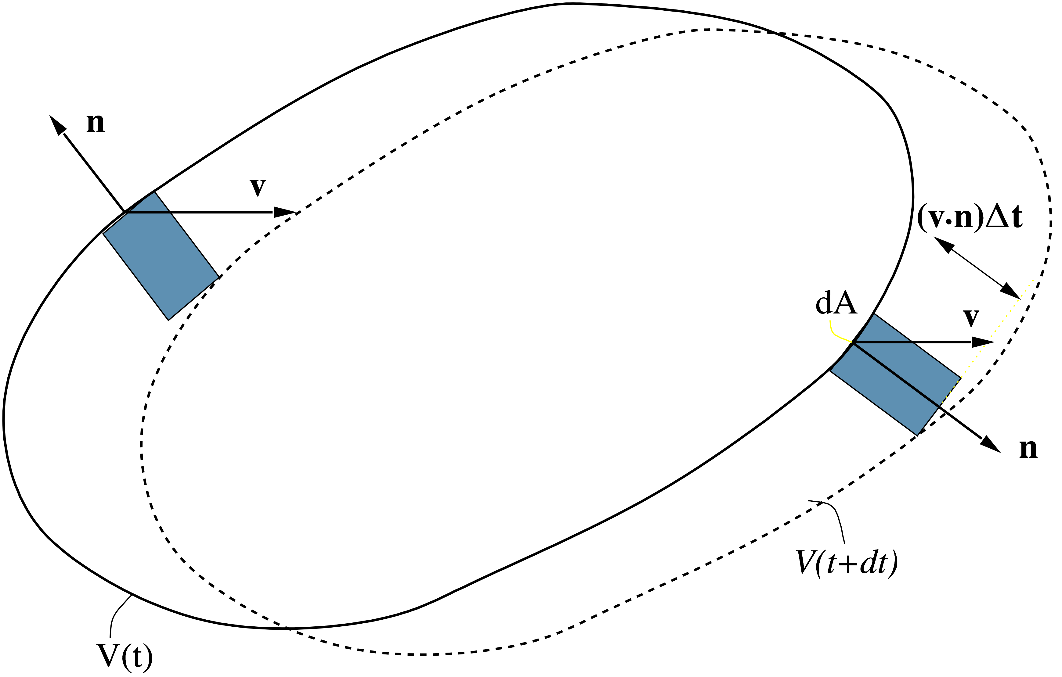
Figure 2: Control volume at time \( t \) and \( t+ \Delta t \).
The fundamental conservation laws (mass, momentum, energy) contain material derivatives of both intensive and extensive properties. In the following the RTT will be derived.
For convenience we introduce the density \( b=\rho \beta \) of an extensive property \( B \) with a corresponding body of volume V(t) and surface area A(t) (Figure 2): $$ \begin{equation} B(t) = \Int_{V(t)} b(\mathbf{r},t) \, dV \tag{2.26} \end{equation} $$ The volume \( V(t) \) may be thought of as the volume of the system or the system of particles, which at a given point in time has the extensive property \( B \). The outset for the derivation, is the canonical definition of a derivative: $$ \begin{equation} \dot{B}\equiv \frac{dB}{dt} = \lim_{\Delta t \rightarrow 0} \frac{B(t+\Delta t) -B(t)}{\Delta t} \tag{2.27} \end{equation} $$ Further, \( B(t+\Delta t) \) must be expanded: $$ \begin{align} B(t+\Delta t) &= \int_{V(t+\Delta t)} b(\mathbf{r},t+\Delta t)\, dV \nonumber \\ &= \int_{V(t)} b(\mathbf{r},t+\Delta t)\, dV + \int_{\Delta V} b(\mathbf{r},t+\Delta t)\, dV \nonumber \end{align} $$ The last integral may be expressed by a surface integral: $$ \begin{equation} \int_{\Delta V} b(\mathbf{r},t+\Delta t)\, dV = \int_{A(t)} b(\mathbf{r},t+\Delta t) \, (\mathbf{v \cdot n} \, \Delta t ) \, dA \tag{2.28} \end{equation} $$ Here, \( \mathbf{v} \) is the velocity of the moving body and \( \mathbf{n} \) is the outward unit normal.
By collection terms: $$ \begin{equation} \frac{B(t+\Delta t) -B(t)}{\Delta t} = \Int_{V(t)} \frac{b(\mathbf{r},t+\Delta t)-b(\mathbf{r},t)}{\Delta t} \, dV + \Int_{A(t)} b(\mathbf{r},t+\Delta t) \, (\mathbf{v \cdot n}) \, dA \tag{2.29} \end{equation} $$ By letting \( \Delta t \rightarrow 0 \) the Reyonlds transport theorem is obtained:
The expression in equation (2.30) is also frequently referred to as Leibniz's rule for 3D integrals (see equation (8.45)).
In some applications, in particular fluid-structure interaction applications, the governing equations have to be formulated on grids which are deforming, but at a different velocity than the fluid/structure. In such cases it is beneficial to introduce a control volume \( V_c(t) \) which deforms at a velocity \( \boldsymbol{v}_c(t) \). An extensive property \( B_c(t) \) may then be introduced in the natural manner: $$ \begin{equation} B_c(t) = \Int_{V_c(t)} b(\mathbf{r},t) \, dV \tag{2.31} \end{equation} $$ Note, that \( B_c \) is not related to the system (or system of particles), but rather to the control volume \( V_c \). In general we have \( B_c(t) \neq B(t) \) whenever \( V_c(t) \neq V(t) \), and thus \( B_c \) is normally not the quantity of interest whenever governing equations for physical phenomena are to be developed. However, we may compute the time derivative of \( B_c \) by using the Reynolds transport theorem in equation (2.30) and note that in this particular instance velocity with which the surface is deforming is \( \boldsymbol{v}_c \), i.e., the velocity of the control volume surface: $$ \begin{equation} \dot{B_c} = \frac{dB_c}{dt} = \Int_{V_c(t)} \partd{b}{t} \, dV + \Int_{A_c(t)} b \, (\mathbf{v}_c \cdot \mathbf{n}) \, dA \tag{2.32} \end{equation} $$ By subtracting equation (2.32) from equation (2.30), rearranging and introducing the definition of \( B_c \), we obtain a version of the Reynolds transport theorem for a moving control volume \( V_c \):
Note, that we tacitly assume that \( V_c(t) = V(t) \) at time \( t \) to derive equation (2.33).
2.1.4 The material derivative of an extensive property
Based on conservation of mass (i.e., \( \dot{\rho \, J}=0 \)) it may be shown that for a generic specific intensive property cite[Theorem C.11]{irgens08} that: $$ \begin{equation} \dot{B} = \ddt \Int_{V(t)} \beta \, \rho \, dV = \Int_{V(t)} \dot{\beta} \, \rho \, dV \tag{2.34} \end{equation} $$