2.5 Stress analysis
From Cauchy's stress theorem ((2.65)) we may compute a stress vector, normal stress, and shear stress on an arbitrary plane with normal \( \mathbf{n} \) in a point/particle \( P \), whenever the stress tensor in known. Below we will simply state without proof a theorem, which will prove useful to identify maximum stresses and planes without shear stress, for generic stress state.
2.5.1 Principal stresses
The shear stress free planes are referred to as principal planes, with corresponding principal directions \( \mathbf{n} \), and principal stresses \( \sigma \). As the principal planes are shear stress free, the stress vector on a principal plane may be expressed by \( \mathbf{t=\sigma n} \), i.e., the stress vector is parallel with the normal vector on the principal plane. By substitution of \( \mathbf{t=\sigma n} \) into (2.65)), the identification of principal stresses and principal directions is reduced to the eigenvalue problem: $$ \begin{equation} \tag{2.115} \mathbf{T} \cdot \mathbf{n} = \sigma \mathbf{n} \end{equation} $$ where the stress-matrix \( \mathbf{T} \) real and symmetric \( \mathbf{T} = \mathbf{T}^T \) (see (2.93). Equivalent representations of the eigenvalue problems in (2.115) are: $$ \begin{equation} \tag{2.116} \left ( \sigma \mathbf{I} - \mathbf{T} \right ) \cdot \mathbf{n} = 0 \qquad \Leftrightarrow \left (\sigma \delta_{ik} - T_{ik} \right ) \; n_k \end{equation} $$ where the latter component form follows is perhaps most easily realized as \( \sigma n_i= \sigma \delta_{ik} n_{k} \) and \( \delta_{ik} \) are the components of the unit matrix \( \mathbf{I} \). For a given principal stress \( \sigma \), (2.116) form a set of three linear, homogenous equations for the three components \( n_k \) of the corresponding principal direction. The condition that (2.116) has a solution, is that the determinant of the coefficient matrix is equal to zero: $$ \begin{equation} |\sigma \delta_{ik} - T_{ik} | = 0 \Rightarrow \left | \begin{array}{ccc} \sigma - T_{11} & -T_{12} & -T_{13} \\ -T_{21} & \sigma -T_{22} & -T_{23} \\ -T_{31} & -T_{32} & \sigma - T_{33} \end{array} \right | = \sigma^3 -I_1 \sigma^2 + I_2 \sigma - I_3 = 0 \tag{2.117} \end{equation} $$
According to conventions, we have introduced the principal invariants of the stress tensor: $$ \begin{align} I_1 &= T_{kk} = \tr \mathbf{T} \tag{2.118} \\ I_2 & = \frac{1}{2} \left ( T_{ii} T_{kk} - T_{ik}T_{ik} \right ) = \frac{1}{2} \left [ (\tr\mathbf{T})^2 - \| \mathbf{T} \|^2 \right ] \tag{2.119} \\ I_3 & = \det \mathbf{T} \tag{2.120} \end{align} $$
The cubic (2.117) is called the characteristic equation of the stress tensor. As \( \mathbf{T} \) is real and symmetric, it follows from basic linear algebra that the three principal stresses \( \sigma_1 \ldots \sigma_3 \) (eigenvalues) , are real, and when distinct, the corresponding principal planes (eigenvectors) are orthogonal. For convenience, the principal stresses may be ordered by their numerical values such that: $$ \begin{equation} \tag{2.121} \sigma_3 \leq \sigma_2 \leq \sigma_1 \end{equation} $$ The fact that any cubic equation with real coefficients, such as (2.117), has a least one real root, may be realized by the following. Let \( f(\sigma) \) denote the left hand side of (2.117). Then, \( f(\sigma) \rightarrow - \infty \) when \( \sigma \rightarrow - \infty \) and \( f(\sigma) \rightarrow \infty \) when \( \sigma \rightarrow \infty \). Thus, there is a least one \( \sigma=\sigma_3 \) for which \( f(\sigma=\sigma_3)=0 \). For principal stress \( \sigma=\sigma_3 \) the corresponding principal direction \( \mathbf{n}_3 \) may be found from (2.116). Now, for convenience, select a coordinate system such that \( \mathbf{e}_3 = \mathbf{n}_3 \). In this coordinate system the corresponding stress vector \( \mathbf{t}_3 = \sigma_3 \, \mathbf{n}_3 \) and \( T_{\alpha3} = 0 \), and the stress matrix is: $$ \begin{equation} \mathbf{T} = \left [ \begin{array}{ccc} T_{11} & T_{12} & 0 \\ T_{21} & T_{22} & 0 \\ 0 & 0 & \sigma_3 \\ \end{array} \right ] \tag{2.122} \end{equation} $$ For this choice of coordinate system, (2.116), simplifies to (note that \( n_3 \) denotes the component in the \( \mathbf{e}_3 \)-direction, for all principal directions \( \mathbf{n}_1 \), \( \mathbf{n}_2 \), and \( \mathbf{n}_3 \).) : $$ \begin{align} \left (\sigma \delta_{\alpha \beta} - T_{\alpha \beta} \right ) \,n_\alpha = 0, \qquad (\sigma -\sigma_3) \,n_3 =0 \tag{2.123} \end{align} $$ By initially assuming that \( \sigma \neq \sigma_3 \) we get from (2.123) that \( n_3=0 \), i.e., the principal directions \( \mathbf{n}_1 \) and \( \mathbf{n}_2 \), will be parallel to the \( x_1 x_2 \)-plane, and normal to \( \mathbf{n}_3 \). The first two equations in (2.123) may be represented in matrix form as: $$ \begin{equation} \left [ \begin{array}{cc} \sigma-T_{11} & -T_{12} \\ -T_{21} & \sigma-T_{22} \end{array} \right ] \left [ \begin{array}{c} n_1 \\ n_2 \end{array} \right ] = 0 \tag{2.124} \end{equation} $$ the corresponding determinant has to be zero for (2.124) to hold for all choices of \( n_1 \) and \( n_2 \): $$ \begin{align} (\sigma-T_{11})(\sigma-T_{22})-T_{12}T_{21} = \sigma^2 - (T_{11} + T_{22}) \sigma + T_{11}T_{22} + T_{12}^2 = 0 \tag{2.125} \end{align} $$ where the latter equality follow from the symmetry of \( \mathbf{T} \), i.e., \( T_{12}=T_{21} \). The solution of the quadratic equation for the determinant is given by: $$ \begin{align} \tag{2.126} \sigma_{1,2} = \frac{1}{2} \left (T_{11} + T_{22} \right ) \pm \sqrt{\left (\frac{T_{11}-T_{22}}{2} \right )^2 + T_{12}^2 } \end{align} $$ The two solutions \( \sigma_1 \) and \( \sigma_2 \) will always be real as the radicand of (2.126) never will be negative. Subject to the condition that the \( \mathbf{e}_3 \)-direction is aligned with the third principal direction \( \mathbf{n}_3 \), (2.126) offers a simple formula to compute the principal stresses. This is very useful for planar states of stress (the section 2.5.3 Planar stress).
If we let \( \phi \) denote the angle between a normal vector \( \mathbf{n} \) and the \( x_1 \)-axis, we can express the components of \( \mathbf{n} \) as: $$ \begin{align} \mathbf{n} = [\cos\phi, \sin\phi,0] \tag{2.127} \end{align} $$ The corresponding principal direction to the eigenvalue \( \sigma_{\alpha} \), may be found by substitution of (2.127) into (2.124), an operations which yields two equations out of which the first one reads: $$ \begin{align} (\sigma_{\alpha} -T_{11} ) \cos \phi_{\alpha} - T_{12} \sin \phi_{\alpha} = 0 \tag{2.128} \end{align} $$ and thus the corresponding principal direction to \( \sigma_{\alpha} \) is given by: $$ \begin{align} \tan \phi_{\alpha} = \frac{\sigma_{\alpha} - T_{11}}{T_{12}} \tag{2.129} \end{align} $$
For a coordinate system aligned with the principal directions, which we denote a principal coordinate system, the stress matrix \( \mathbf{T} \) takes the form,: $$ \begin{equation} \mathbf{T} = \left [ \begin{array}{ccc} \sigma_1 & 0 &0 \\ 0 & \sigma_2 &0 \\ 0 & 0 & \sigma_3 \end{array} \right ] \quad \Leftrightarrow \quad T_{ik} = \sigma_i \delta_{ik} \quad \text{no sum over i} \tag{2.130} \end{equation} $$ and then an equivalent, but simpler representation of the principal invariants may be found as: $$ \begin{align} I_1 & = \sigma_1 + \sigma_2 + \sigma_3 \tag{2.131} \\ I_2 & = \sigma_1\sigma_2 + \sigma_2 \sigma_3 + \sigma_3 \sigma_1 \tag{2.132}\\ I_3 & = \sigma_1 \sigma_2 \sigma_3 \tag{2.133} \end{align} $$ Thus, in (2.131) and (2.133), the principal invariants are expressed by the principal stresses, whereas in (2.118) - (2.120) they are expressed by the coordinate stresses.
For a principal coordinate system, the normal stress \( \sigma \) on a plane with unit normal \( \mathbf{n} \) is given by: $$ \begin{equation} \sigma = \mathbf{n\cdot T \cdot n} = \sum_{i,k} n_i \sigma_i \delta_{ik} n_k = \sigma_1 n_1^2 + \sigma_2 n_2^2 + \sigma_3 n_3^2 \tag{2.134} \end{equation} $$ From (2.134), the ordering in (2.121) and the property of a unit normal vector \( \mathbf{n \cdot n} = n_1^2 + n_2^2 + n_3^2 = 1 \) , one may find that: $$ \begin{equation} \sigma_3 \left (n_1^2 + n_2^2 + n_3^2 \right ) \leq \sigma \leq\sigma_1 \left ( n_1^2 + n_2^2 + n_3^2 \right ) \quad \Rightarrow \quad \sigma_3 \leq \sigma \leq \sigma_1 \tag{2.135} \end{equation} $$ Thus, as (2.135) must hold for any \( \mathbf{n} \), the extremal normal stresses \( (\sigma_{\max},\sigma_{\min}) \) are given by: $$ \begin{equation} \sigma_{\max} = \sigma_1, \qquad \sigma_{\min} = \sigma_3 \tag{2.136} \end{equation} $$ The largest principal stress \( \sigma_1 \), is therefore the maximum normal stress on any planes at a given location/particle. Correspondingly, \( \sigma_3 \) is the minimum normal stress on any planes at a given location/particle, whereas \( \sigma_2 \) is called the intermediate principal stress.
Extremal normal stresses The extremal normal stresses are given by the principal stresses \( \sigma_1 \) and \( \sigma_3 \).
2.5.2 Maximum shear stress
Figure 11: Shear stress \( \tau \) and normal stress \( \sigma \) in planes parallel to \( \mathbf{n}_2 \).

The component \( \tau \) in an arbitrary direction \( \mathbf{e} \) of the stress vector \( \mathbf{t} \) acting on a surface with orientation \( \mathbf{n} \) is given by (2.84): $$ \begin{equation} \tau = \mathbf{e} \cdot \mathbf{t}= e_i T_{ik} n_k = \sum_{i,k} e_i \sigma_i \delta_{ik} n_k = \sigma_1 e_1 n_1 + \sigma_2 e_2 n_2 + \sigma_3 e_3 n_3 \tag{2.137} \end{equation} $$ The latter expression in (2.137), follow by assuming a principal coordinate system with a stress matrix given by (2.130). Now, by choosing \( \mathbf{e} \) to be orthogonal to \( \mathbf{n} \), i.e., computing the shear stress which is the component of the stress vector \( \mathbf{t} \) in the plane which has \( \mathbf{n} \) as normal vector: $$ \begin{equation} \mathbf{e\cdot n} = e_i \; n_i = 0 \qquad\Rightarrow \qquad e_2 n_2 = -e_1 n_1 - e_3 n_3 \tag{2.138} \end{equation} $$ Substituting (2.138) into (2.137) we get: $$ \begin{equation} \tau = (\sigma_1 -\sigma_2) \; e_1n_1 - (\sigma_2 -\sigma_3) \; e_3n_3 \tag{2.139} \end{equation} $$ Due to the ordering in (2.121), the expressions in the parenthesis of (2.139) will always be positive. Thus, in order to maximize \( \tau \), the expressions \( e_1n_1 \) and \( -e_3n_3 \) must be taken as large as possible. The absolute of \( e_1 \), \( n_1 \), \( e_3 \), and \( n_3 \) become largest if \( e_2=n_2=0 \), as \( \mathbf{e} \) and \( \mathbf{n} \) are orthogonal unit vectors. In other words, to find the maximum shear stress we should choose \( \mathbf{e} \) and \( \mathbf{n} \) in a plane parallel to the plane spanned by the principal directions \( \mathbf{n}_1 \) and \( \mathbf{n}_3 \). Equivalently, the plane with orientation \( \mathbf{n} \), should be parallel to the \( \mathbf{n}_2 \) principal direction (Figure 11). Note that since \( \mathbf{n}_2 \) is a principal direction, the stress vector \( \mathbf{t} \) in Figure 11 has no component in the \( \mathbf{n}_2 \)-direction. Letting \( \phi \) denoting the angle in the counter clockwise direction with respect to the first principal direction \( \mathbf{n}_1 \), we may deduce from Figure 11: $$ \begin{equation} n_1 = \cos \phi = -e_3 \qquad \text{and} \qquad e_1 = \sin\phi = n_3 \tag{2.140} \end{equation} $$ By substituting (2.140) into (2.139), we realize that the \( \sigma_2 \)-terms cancel and that the shear stress may be represented: $$ \begin{equation} \tau = (\sigma_1 - \sigma_3) \cos \phi \sin \phi = \frac{1}{2} \, (\sigma_1 - \sigma_3) \sin 2\phi \tag{2.141} \end{equation} $$ the latter relation follow from the trigonometric formula (8.2).
Thus, the shear stress has its maximum value \( \tau_{\max} \), for \( \phi=\pi/4 \), and $$ \begin{equation} \tau_{\max} = \frac{1}{2} \, (\sigma_{\max} - \sigma_{\min}) \tag{2.142} \end{equation} $$
which is a generic important result:
The maximum shear stress
The maximum shear stress acts on planes that are inclined \( 45^ {\circ} \) with respect to the principal directions of the maximum and minimum principal stresses.
This result may also be obtained by considering a cube is aligned with the principal directions (Figure 12, upper panel). Consider a cross-section parallel with \( \mathbf{n}_2 \), tilted with an angle \( \phi \) with respect to the \( \mathbf{n}_3 \)-direction (Figure 12, lower panel).
Figure 12: A cube aligned with the principal directions.
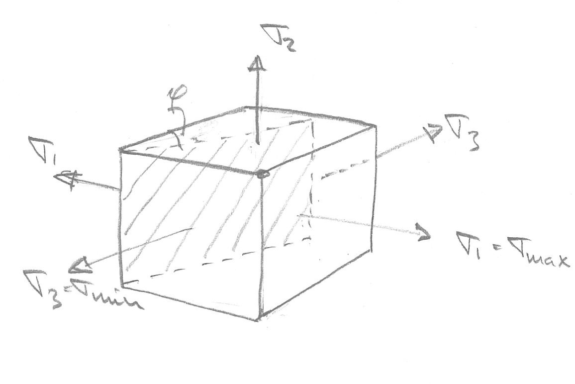
Figure 13: Max shear stress illustration.

On such a surface there will be a normal stress \( \sigma \) and shear stress \( \tau \), to satisfy equilibrium (balance of linear momentum). Without loss of generality, the length of the tilted edge in Figure 13 (lower panel), is taken to be unity.
We then find an expression for the shear stress by balancing the forces in the \( \tau \)-direction: $$ \begin{equation} \tau + \sigma_3 \cos \phi \sin \phi - \sigma_1 \sin \phi \cos \phi = 0 \tag{2.143} \end{equation} $$ which provides an expression for the shear stress \( \tau \): $$ \begin{equation} \tau = (\sigma_1 - \sigma_3) \sin \phi \cos \phi = \frac{1}{2} \sin 2\phi\, (\sigma_1 - \sigma_3) \tag{2.144} \end{equation} $$ which is identical to (2.141) and leads to (2.142).
The corresponding normal stress \( \sigma \) may be found by fulfillment of the equilibrium criterion in the normal direction: $$ \begin{equation} \sigma - \sigma_1 \cos^2 \phi - \sigma_3 \sin^2 \phi = 0 \tag{2.145} \end{equation} $$ which at \( \phi=\pi/4 \) yields: $$ \begin{equation} \sigma = \frac{1}{2} \, (\sigma_1 + \sigma_3) \tag{2.146} \end{equation} $$
2.5.3 Planar stress
If there is a stress free plane for a given stress state, we say that the structure/particle is in a state of plane stress or equivalently a state of biaxial stress. In particular for extreme loads, this is often the case in engineering/bioengineering application. Even when the surface is loaded, a planar stress assumption may serve as a good first approach, as will be seen for thin-walled spheres and cylinders in example 2.5.4 Example 6: Biaxial state of stress for thin-walled structures.
For a planar stress situation, we may select a coordinate system such that the z-axis is orthogonal to the stress free plane. Consequently, all stress components in the \( z \)-direction will be zero: \( \sigma_z = \tau_{xz} = \tau_{yz} = 0 \). Therefore, the \( xy \)-plane is a principal plane with corresponding principle stress \( \sigma_3 = \sigma_z = 0 \), and the stress matrix in (2.60) reduces to: $$ \begin{equation} \mathbf{T} = \left [ \begin{array}{cc} \sigma_x & \tau_{xy} \\ \tau_{xy} & \sigma_y \end{array} \right ] \tag{2.147} \end{equation} $$
In the following we will present two ways to derive the expressions for the stresses \( \sigma \) and \( \tau \) on a plane parallel to the z-axis, for an arbitrary plane with a unit normal \( \mathbf{n} \) at angle \( \phi \) with respect to the \( x \)-axis. First, we will use the generic expressions for \( \sigma \) and \( \tau \) as presented in Eqs. (2.134) and (2.137).
Figure 14: Planar stress situation.

A generic planar stress situation is illustrated in Figure 14 and the unit normal and the unit tangent vectors may be expressed by: $$ \begin{align} \mathbf{n} &= [\cos \phi, \sin \phi] \tag{2.148}\\\mathbf{e} &= [\sin \phi, -\cos \phi] \tag{2.149} \end{align} $$
From CST in (2.65) we get: $$ \begin{equation} t_{\alpha} = T_{\alpha\beta} n_{\beta} \tag{2.150} \end{equation} $$ and by use of the stress matrix in (2.147) we get: $$ \begin{align} t_1& = \sigma_x \cos \phi + \tau_{xy} \sin \phi \tag{2.151}\\ t_2& = \tau_{xy} \cos \phi + \sigma_y \sin \phi \tag{2.152} \end{align} $$ Now, the normal stress \( \sigma \) an the shear stress \( \tau \) are found from Eqs. (2.134) and (2.137): $$ \begin{align} \sigma & = \mathbf{n \cdot t} = n_{\alpha} t_{\alpha} = \sigma_x \cos^2 \phi + \sigma_y \sin^2 \phi + 2 \tau_{xy} \sin \phi \cos \phi \tag{2.153}\\ \tau &= \mathbf{e \cdot t} = e_{\alpha} t_{\alpha} = \left (\sigma_x - \sigma_y \right ) \sin \phi \cos \phi- \tau_{xy} \left ( \cos^2\phi - \sin^2\phi \right ) \tag{2.154} \end{align} $$
Now, by making use of the trigonometric relations in (8.2), the expressions for the normal and shear stress at an arbitrary plane given by (2.153) and (2.154) may be simplified to: $$ \begin{align} \sigma(\phi) & = \frac{\sigma_x + \sigma_y}{2} + \frac{\sigma_x - \sigma_y}{2} \cos 2 \phi + \tau_{xy} \sin 2\phi \tag{2.155}\\ \tau(\phi) & = \frac{\sigma_x - \sigma_y}{2} \sin 2 \phi - \tau_{xy} \cos 2\phi \tag{2.156} \end{align} $$ The second way of derving the expressions in (2.155) and (2.156), for the normal stress \( \sigma \) and the shear stress \( \tau \), is to formulate expressions which meet the requirement of force equilibrium in two perpendicular directions. The expression for the normal stress \( \sigma \) is obtained from the requirement of force equilibrium in the \( \mathbf{n} \)-direction (Figure 14): $$ \begin{equation} \sigma(\phi) \cdot 1 - \sigma_x \cos^2\phi - \sigma_y \sin^2\phi - \tau_{xy}\sin\phi\cos\phi - \tau_{xy}\cos\phi\sin\phi = 0 \tag{2.157} \end{equation} $$ which may be reorganized to the previously derived expressions for the normal stress \( \sigma(\phi) \) as given by Eqs. (2.153), (2.154), (2.155), and (2.156). Similarly, an expression for the shear stress \( \tau \) is obtained from the requirement of force equilibrium in the \( \tau \)-direction: $$ \begin{equation} \tau(\phi) \cdot 1 - \sigma_x \sin\phi\cos\phi + \sigma_y \cos\phi\sin\phi + \tau_{xy} \cos^2\phi - \tau_{xy}\sin^2\phi =0 \tag{2.158} \end{equation} $$ which also may be reorganized to the previously derived expressions for the shear stress as given by Eqs. (2.153), (2.154) and (2.156).
For a planar state of stress, one may orient a coordinate system with the \( x_3 \)-direction perpendicular to the stress free plane. Thus, \( \mathbf{e}_3 \) is a principal direction, with a known principal stress \( \sigma_3=0 \). We may then use the perviously derived, generic expressions for the principal stresses in Eqs. (2.126) and (2.129), for the normal stress values in a planar state of stress. We repeat them here, using engineering notation: $$ \begin{align} \tag{2.159} \sigma_{1,2}& = \frac{1}{2} \left (\sigma_x + \sigma_y \right ) \pm \sqrt{\left (\frac{\sigma_x-\sigma_y}{2} \right )^2 + \tau_{xy}^2 }\\ \tag{2.160} \tan \phi_{\alpha} &= \frac{\sigma_{\alpha} - \sigma_x}{\tau_{xy}} \end{align} $$ Note that \( \sigma_1 \) and \( \sigma_2 \) may both be positive, or both be negative, or have different signs. Thus, the conventional ordering of \( \sigma_3 \leq \sigma_2 \leq \sigma_1 \), is not adopted for planar states of stress, as \( \sigma_3 = 0 \) is tacitly assumed while employing (2.159). Keeping this in mind, (2.142) is still valid for the calculation of the maximum shear stress for a planar state of stress: $$ \begin{align} \tau_{\max} = \frac{1}{2} \, (\sigma_{\max} - \sigma_{\min}) \tag{2.161} \end{align} $$ where: $$ \begin{align} \sigma_{\max} = \max(0,\sigma_1), \qquad \sigma_{\min} = \min(0,\sigma_2) \tag{2.162} \end{align} $$
2.5.4 Example 6: Biaxial state of stress for thin-walled structures
In this example we will consider two typical planar or biaxial states of stress, resulting from a thin-walled assumption. As we will see, this assumption has the convenient consequence, that one of the normal stress components is much smaller than the two others.First we consider a thin-walled spherical shell (Figure 15) subjected to an internal pressure \( p \). The mid wall radius of the shell is \( r \), and the wall thickness is \( t \ll r \). We conveniently select a spherical coordinate system \( (r,\theta,\phi) \), which is also a principal coordinate system for the current state of stress.
Figure 15: A free-body diagram of a hemisphere.
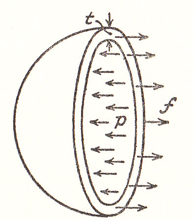
Figure 16: A free-body diagram of a circular cylinder.

To meet the requirement of equilibrium of forces for two perpendicular cross-sections at the equator, with orientation \( \mathbf{e}_{\phi} \) and \( \mathbf{e}_{\theta} \), respectively, the following equations must be satisfied: $$ \begin{equation} p \pi r^2 = \sigma_{\theta} 2 \pi r t = \sigma_{\phi} 2 \pi r t \tag{2.163} \end{equation} $$ from which the expressions for the average wall stresses \( \sigma_{\phi} \) and \( \sigma_{\theta} \), may be derived: $$ \begin{equation} \sigma_{\phi} = \sigma_{\theta} =\frac{1}{2} \frac{r}{t} p \tag{2.164} \end{equation} $$
The Eqs. (2.164) are commonly referred to as the Laplace equations. The remaining stress \( \sigma_r \) in the \( r \)-direction must be in the range \( [-p,0] \) to meet the requirement of equilibrium. Thus from the thin-walled assumption (\( t \ll r \)) and Eqs. (2.164) we find that \( \sigma_r \ll \sigma_{\phi} = \sigma_{\theta} \). Consequently, \( \sigma_r \) may be disregarded for the stress analysis of a thin-walled spherical shell. The stress state may be regarded as planar or biaxial with the following the stress matrix: $$ \begin{equation} \mathbf{T} = \left [ \begin{array}{ccc} 0 & 0 & 0 \\ 0 & 1 & 0 \\ 0 & 0 & 1 \end{array} \right ] \frac{1}{2} \frac{r}{t} p \tag{2.165} \end{equation} $$ in a spherical coordinate system, which is seen to be a principal coordinate system, as there are no shear stresses present in the stress matrix of (2.165). We observe the common property of thin-walled structures, namely, that two stress components scale with \( r/t \) and \( p \), \ie $$ \begin{align} \sigma_{\phi,\theta} \propto \frac{r}{t} \; p \tag{2.166} \end{align} $$ whereas the third stress component \( \sigma_{r} \), scales with \( p \) only, and may consequently be disregarded.
Further, any direction parallel to the shell surface is a principal direction, since the stresses in the \( \phi \)- and the \( \theta \)-directions are equal. The state of stress for the thin-walled spherical shell may therefore be referred to as biaxial and plane-isotropic.
The second thin-walled structure we consider in this example, is a circular cylinder loaded with an internal pressure \( p \) (see Figure 16). The mid wall radius of the cylinder is \( r \), and the wall thickness is \( t \ll r \). Analogous to the spherical shell, we conveniently select a cylindrical coordinate system \( (r,\theta,z) \), which is also a principal coordinate system for the current state of stress.
To meet the requirement of equilibrium of forces for a perpendicular cross-sections at the equator, with orientation \( \mathbf{e}_{r} \) the following equations must be satisfied: $$ \begin{equation} 2 \, \sigma_{\theta} \Delta z \, t = p \, 2 r \Delta z \tag{2.167} \end{equation} $$ and an expression for \( \sigma_{\theta} \), commonly referred to as the hoop stress, is obtained: $$ \begin{equation} \sigma_{\theta} = \frac{r}{t} \, p \tag{2.168} \end{equation} $$ For a cross-section with orientation \( \mathbf{e}_z \), the requirement of force equilibrium yields the same value as for the sphere in (2.163): $$ \begin{equation} \sigma_z =\frac{1}{2} \frac{r}{t} p \tag{2.169} \end{equation} $$ Again, as for the thin-walled sphere, the remaining stress \( \sigma_r \) in the \( r \)-direction must be in the range \( [-p,0] \) to meet the requirement of equilibrium. From the thin-walled assumption (\( t \ll r \)) and Eqs. (2.168) and (2.169) we find that \( \sigma_r \ll \sigma_{\phi} = 2\, \sigma_{z} \). We observe that the stresses for a thin-walled cylinder conform to the generic stress state of a thin-walled structure in (2.166). Consequently, \( \sigma_r \) may be disregarded for the stress analysis of a thin-walled circular cylinder and the stress state may be regarded as planar or biaxial with the following the stress matrix in a cylindrical, principal coordinate system: $$ \begin{equation} \mathbf{T} = \left [ \begin{array}{ccc} 0 & 0 & 0 \\ 0 & 2 & 0 \\ 0 & 0 & 1 \end{array} \right ] \frac{1}{2} \frac{r}{t} p \tag{2.170} \end{equation} $$
Observe, that the thin-walled circular cylinder is statically determinate, i.e., the stress state may be found from equilibrium analysis alone. On the contrary, a thick-walled cylinder is statically indeterminate, which has the consequence that the material properties of the wall has to be accounted for to determine the state of stress.