5.4 Linear viscous fluids

Figure 37: Cylindrical viscometer.

Viscous fluids Fluid particles are slowed down in the vicinity of a solid wall (see Figure 36). Shear stresses are present wherever there are velocity gradients. The influence of (wall) shear stresses (WSS) are most prominent in the vicinity of solid walls.

Flow around rigid bodies. External flow field modeled as a perfect fluid. BL flow near the rigid surface with asymptotic external flow.

The velocity field for simple shear flow $$ \begin{equation} v_1 = \frac{v}{h} x_2, v_2=v_3 = 0 \tag{5.35} \end{equation} $$ Strain rate $$ \begin{equation} \dot{\gamma} = 2 D_{12} = \frac{dv_1}{dx_2} = \frac{v}{h} = \frac{\omega r}{h} \tag{5.36} \end{equation} $$ Shear stress from torque T $$ \begin{align} (\tau r) ( 2\pi r H) &= T \tag{5.37}\\ \tau = \frac{T}{2\pi r^2 H} \tag{5.38} \end{align} $$

5.4.1 Simple shear flow

Figure 38: Illustration of simple shear flow between two parallel planes.

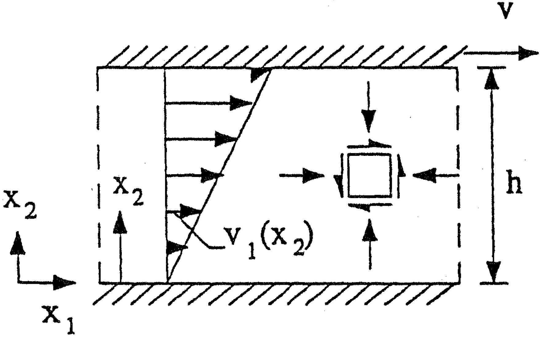
Figure 39: Illustration of the shear rate for a small fluid element in a simple shear flow.

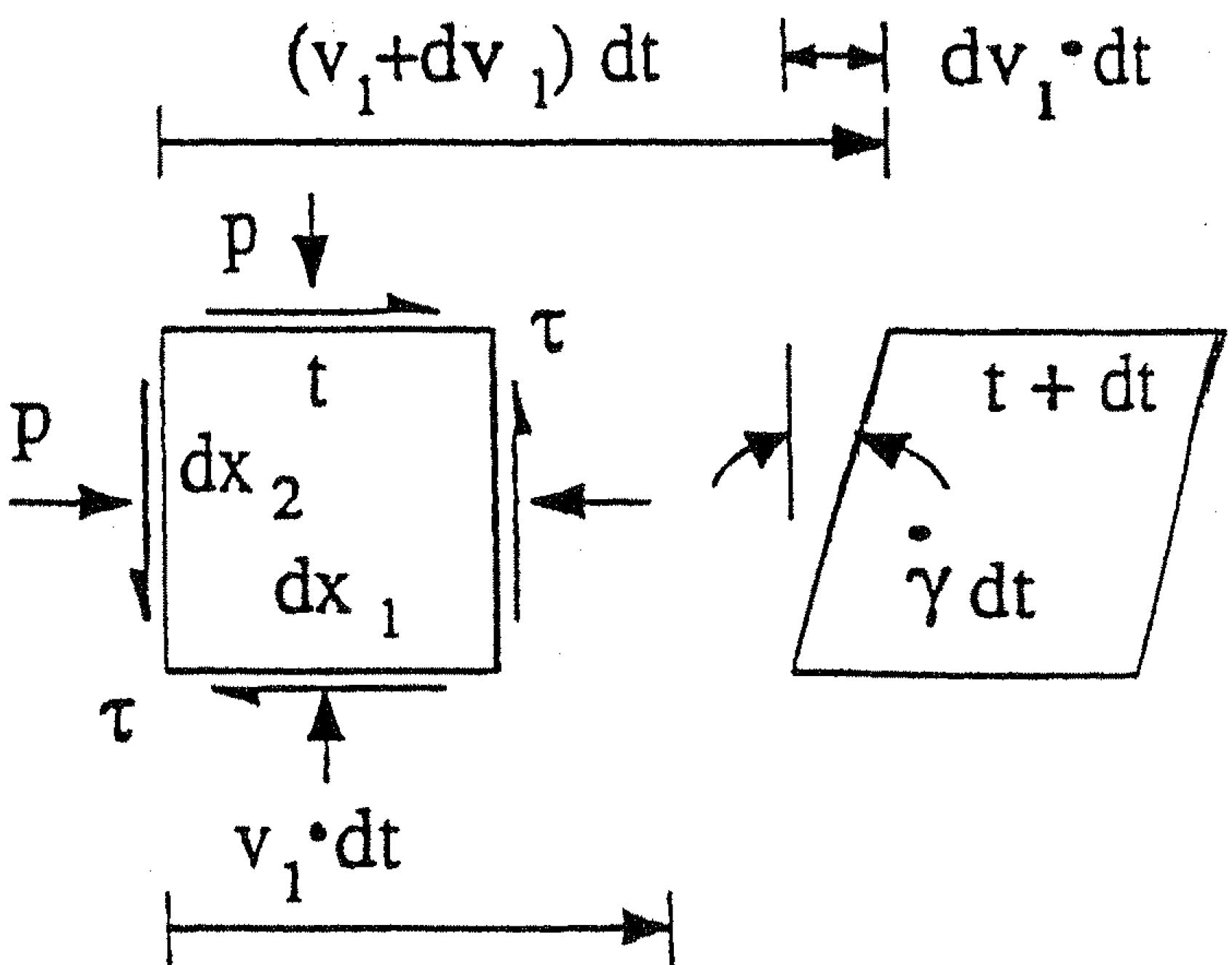
The velocity field $$ \begin{equation} v_1 = \frac{v}{h} x_2, v_2=v_3 = 0 \tag{5.39} \end{equation} $$ The rate of deformation $$ \begin{equation} \boldsymbol{D} = \left [ \begin{array}{ccc} 0 & 1 & 0 \\ 1 & 0 & 0 \\ 0 & 0 & 0 \end{array} \right ] \, \frac{\dot{\gamma}}{2} \tag{5.40} \end{equation} $$ where: $$ \begin{equation} \dot{\gamma} = \dot{\gamma}_{12} = \boldsymbol{e}_1 \cdot \boldsymbol{D} \cdot \boldsymbol{e}_2 = 2 D_{12} = \frac{dv_1}{dx_2} = \frac{v}{h} \tag{5.41} \end{equation} $$ From experiments: $$ \begin{equation} \tau = \mu \, \dot{\gamma} \tag{5.42} \end{equation} $$

Generalization from simple shear flow From experiments: $$ \begin{equation} \tau = \mu \dot{\gamma} = 2 \mu D_{12} \tag{5.43} \end{equation} $$

Newton's law of fluid friction: $$ \begin{equation} T_{ij} = 2 \mu D_{ij} = \mu (v_{i,j} + v_{j,i}) \quad \mathrm{for} \quad i \neq j \tag{5.44} \end{equation} $$

Stokes' criteria for stress/velocity relation in viscous fluids

$ \boldsymbol{T} $ is a continuous function of $ \boldsymbol{D} $
Homogeneous, i.e., $ \boldsymbol{T} $ independent of particle coordinates
$ \boldsymbol{T}= -p(\rho,\theta) \boldsymbol{1} $ when $ \boldsymbol{D} = 0 $
Viscosity is an isotropic property (redundant)

Newtonian fluid

The Stokes criteria imply a constitutive equation for a Stokes fluid of the form $$ \begin{equation} \boldsymbol{T} = \boldsymbol{T}[\boldsymbol{D},\rho,\theta], \quad \boldsymbol{T}[\boldsymbol{0},\rho,\theta] = -p(\rho,\theta) \boldsymbol{1} \tag{5.45} \end{equation} $$

Linear viscous fluid (Newtonian)

Linear viscous isotropic properties implies that $ \boldsymbol{T} $ and $ \boldsymbol{D} $ are co-axial
The constitutive equation may be shown to be:

$$ \begin{align} \boldsymbol{T} &= -p(\rho,\theta) \boldsymbol{1} + 2\mu \boldsymbol{D} + (\kappa - \frac{2\mu}{3}) \, (\tr \boldsymbol{D}) \, \boldsymbol{1} \tag{5.46}\\ T_{ij} &= -p(\rho,\theta) \delta_{ij} + 2\mu D_{ij} + (\kappa - \frac{2\mu}{3}) \, D_{kk} \, \delta_{ij} \tag{5.47} \end{align} $$

The properties of the Newtonian fluid. Dynamic shear viscosity

$ \mu = \mu(\theta) $ (rarely pressure dependent)
Relatively simple to determine experimentally
$ \mu = 1.8 \cdot 10^{-3} \; \mathrm{Ns/m^2} $ at $ 0^\circ $ C
$ \mu = 1.0 \cdot 10^{-3} \; \mathrm{Ns/m^2} $ at $ 20^\circ $ C
$ \mu = 1.7 \cdot 10^{-5} \; \mathrm{Ns/m^2} $ at $ 0^\circ $ C
$ \mu = 1.8 \cdot 10^{-5} \; \mathrm{Ns/m^2} $ at $ 20^\circ $ C

Bulk viscosity $ \kappa $

Difficult to measure experimentally
Resistance toward rapid volume changes
Incompressible Newtonian fluid

$$ \begin{equation} \boldsymbol{T} = -p(\rho,\theta) \boldsymbol{1} + 2\mu \boldsymbol{D} \tag{5.48} \end{equation} $$

5.4.2 The Navier-Stokes equations

The Navier-Stokes equations

Equations of motion for Newtonian fluids may be derived from Cauchy's equations of motion $$ \begin{equation} \dot{\boldsymbol{v}} = \partd{\boldsymbol{v}}{t} + (\boldsymbol{v} \cdot \nabla) \boldsymbol{v} = \frac{1}{\rho} \nabla \cdot \boldsymbol{T} + \boldsymbol{b} \tag{5.49} \end{equation} $$ and employihg the constitutive equations for a Newtonian fluid: $$ \begin{equation} \boldsymbol{T} = -p(\rho,\theta) \boldsymbol{1} + 2\mu \boldsymbol{D} + (\kappa - \frac{2\mu}{3}) \, (\tr \boldsymbol{D}) \, \boldsymbol{1} \tag{5.50} \end{equation} $$ The Navier-Stokes (NS) equations are obtained by substitution $$ \begin{equation} \partd{\boldsymbol{v}}{t} + (\boldsymbol{v} \cdot \nabla) \boldsymbol{v} = -\frac{1}{\rho} \nabla p + \frac{\mu}{\rho} \, \nabla^2 \boldsymbol{v} % + \frac{1}{\rho} (\kappa + \frac{\mu}{3})\nabla (\nabla \cdot \boldsymbol{v}) + \boldsymbol{b} \tag{5.51} \end{equation} $$ The NS equations for incompressible fluids $$ \begin{equation} \partd{\boldsymbol{v}}{t} + (\boldsymbol{v} \cdot \nabla) \boldsymbol{v} = -\frac{1}{\rho} \nabla p + \frac{\mu}{\rho} \, \nabla^2 \boldsymbol{v} + \boldsymbol{b} \tag{5.52} \end{equation} $$

Figure 40: Flow between parallel planes

Figure 41: Solutions forvarious pressure gradients and upper plane velocities.

5.4.3 About the NS equations

After Claude-Louis Navier and George Gabriel Stokes. The most important equations for viscous fluids. Analytical solutions require major simplifications due to the complexity Models for weather forecasts, ocean currents, pollution, stars in galaxies, aircraft and car design, blood flow. Coupled with Maxwell's equations to model and study magnetohydrodynamics. Coupled with Cauchy's equations for solid materials to study fluid structure interaction problems, e.g., blood and vessel wall. All but the simplest problems must be solved with Computational Fluid Dynamics (CFD) codes

5.4.4 Example 14: Flow between parallel planes

Saint-Venant's semi-inverse method: Unknown functions are partly assumed known. Employ the governing equations and BCs to determine completely.

Assume steady state and velocity field: $$ \begin{equation} v_1 = v_1(y), v_2= v_3=0 \tag{5.53} \end{equation} $$

Incompressibility $ \nabla \cdot \boldsymbol{v} = 0 $. The constitutive equation yields: $$ \begin{equation} T_{11} = T_{22} = T_{33} = -p, \quad T_{12} = \mu v_{1,2} \tag{5.54} \end{equation} $$

Both pressure gradient and upper plate are driving forces for the flow. For convenience $ -p_{,1} = c $.

By substitution of the stress field in Cauchy's equation $$ \begin{align} 0&=c+\mu v_{1,22} \tag{5.55}\\ 0&=-p_{,2} - \rho g \tag{5.56}\\ 0&=-p_{,3} \tag{5.57} \end{align} $$ By integration $$ \begin{align} p &= -\rho g y - c x \tag{5.58}\\ v_1 &= -\frac{c}{2\mu} y^{2} + B y + C \tag{5.59} \end{align} $$ where B and C are constants. BCs $ v_1=0 $ at $ y=0 $ and $ v_1=v $ at $ y=h $ to find constants. The velocity field: $$ \begin{equation} v_1(y) = \frac{c h^{2}}{2 \mu} \left [ \frac{y}{h} - \left (\frac{y}{h} \right )^2 \right ] + v \frac{y}{h} \tag{5.60} \end{equation} $$

5.4.5 Example 15: Laminar pipe flow

Incompressible Newtonian flow. Pipe with diameter $ d $. Flow driven by pressure gradient in z-direction. Laminar, steady flow field $$ \begin{equation} v_z = v(R), \quad v_R=v_{\theta} = 0 \tag{5.61} \end{equation} $$ NS in cylindrical coordinates $$ \begin{align} -\partd{p}{R} = 0, \quad \frac{1}{R} \partd{p}{\theta} &= 0 \tag{5.62}\\ +\frac{1}{R} \partd{}{R} \left ( R \mu \partd{v}{R} \right ) - \partd{p}{z} &= 0 \tag{5.63} \end{align} $$ BCs: $ v(D/2) = 0 $ and $ v(0) \neq \infty $

Figure 42: Laminar pipe flow

Velocity field for laminar pipe flow. Parabolic velocity field: $$ \begin{align} v &= v_0 \left ( 1 - \left (\frac{2R}{d} \right )^2 \right ) \tag{5.64}\\ v_0 &= \frac{d^2}{16 \mu} \, c \tag{5.65}\\ c &= -\partd{p}{z} \tag{5.66} \end{align} $$