5.6 Pulsatile flow in straight tubes
The Navier-Stokes equations for fully developed flow in straight pipes reduce to: $$ \begin{equation} \partd{v}{t} = -\frac{1}{\rho} \partd{p}{z} + \frac{\nu}{r} \partd{}{r} \left ( r \partd{v}{r} \right ) \tag{5.98} \end{equation} $$ By introducing characteristic scales for spatial components \( r^* = r/a \) and \( z^* = z/a \), and for time: \( t^* = t \omega \) and velocity: \( v^* = v/V \) Eq. (5.98) may be cast into a dimensionless form: $$ \begin{equation} \left ( a^2 \frac{\omega}{\nu} \right ) \partd{v^*}{t^*} = - \left (\frac{a}{\rho \nu V} \right ) \partd{p}{z^*} + \frac{1}{r^*} \partd{}{r^*} \left ( r^* \partd{v^*}{r^*} \right ) \tag{5.99} \end{equation} $$ From Eq. (5.99) a natural scale for pressure occurs: $$ \begin{equation} p^* = p/(\rho \nu V / a) = p/(\mu V / a) \tag{5.100} \end{equation} $$ which by substitution into Eq. (5.99) gives the simensionless straight tube equations $$ \begin{equation} \alpha^2 \partd{v^*}{t^*} = - \partd{p^*}{z^*} + \frac{1}{r^*} \partd{}{r^*} \left ( r^* \partd{v^*}{r^*} \right ) \tag{5.101} \end{equation} $$ where the Womersley parameter: $$ \begin{equation} \alpha = a \sqrt{\frac{\omega}{\nu}} \tag{5.102} \end{equation} $$ has been introduced.
Flows where \( \alpha \rightarrow \infty \) are commonly denoted inertia dominated, as viscous forces are negligible compared to the other terms in Eq. (5.101) and the pressure gradient is used solely for acceleration of the fluid mass. Such a situation will typically occur in large vessels, at high frequency flows. In the aorta \( \alpha \ge 20 \).
Similarly, flows where \( \alpha \rightarrow 0 \) (i.e., for small vessels and/or low frequencies) are called friction dominated. In the capillaries \( \alpha = 10 ^{-2} \).
5.6.1 Straight tube velocity profiles
For developed, transient flow in a straight tube the momentum equation reduces to: $$ \begin{equation} \alpha^2 \partd{v}{t} = - \partd{p}{z} + \frac{1}{r} \partd{}{r} \left ( r \partd{v}{r} \right ) \tag{5.103} \end{equation} $$
As (5.103) is linear in \( v \) superposition of solutions for various harmonics is ok. To proceed further, we assume the driving force to be oscillating and represent it by: $$ \begin{equation} \partd{p}{z} = \partd{\hat{p}}{z} e^{i t} \tag{5.104} \end{equation} $$
Due to the harmonic form of the pressure gradient we furhter assume that the velocity may be represented in a similar manner as \( v=\hat{v} e^{i t} \). By substitution into momentum equation (5.103) we get: $$ \begin{equation} i \alpha^2 \hat{v}(r) = - \partd{\hat{p}}{z} + \frac{1}{r} \partd{}{r} \left ( r \partd{\hat{v}}{r} \right ) \tag{5.105} \end{equation} $$
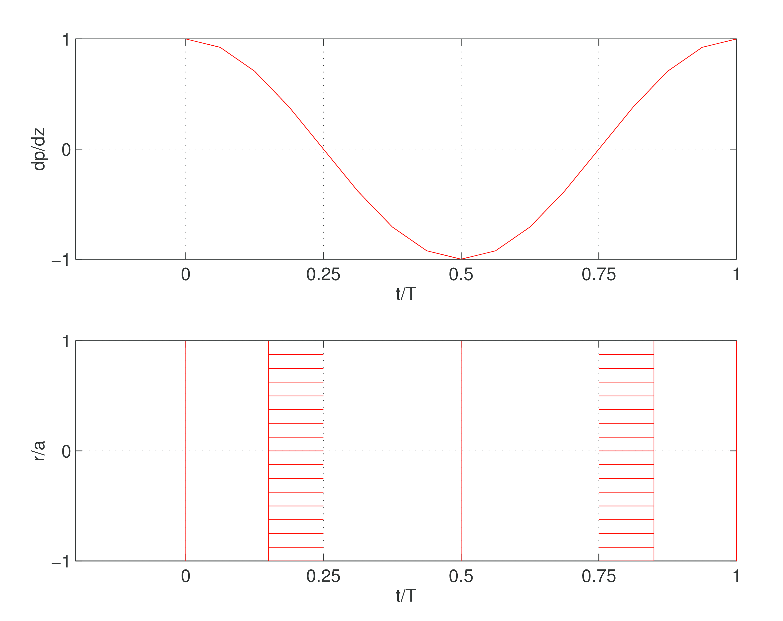
Figure 47: Pressure gradient (upper panel) and velocity profile (lower panel) as a function of time for friction dominated flows [3].

To approach the problem gently we first study the situation of small or vanishing Womersley parameter \( (\alpha \rightarrow 0) \) in (5.103), which corresponds to a situation of friction dominated straight pipe flow. In this situation (5.103) reduces to: $$ \begin{equation} \frac{1}{r} \partd{}{r} \left ( r \partd{\hat{v}}{r} \right ) = \partd{\hat{p}}{z} \tag{5.106} \end{equation} $$
Solution $$ \begin{equation} \hat{v} = -\frac{1}{4}\,\partd{\hat{p}}{z} \left ( 1 - r^2 \right ) \tag{5.107} \end{equation} $$
In the time domain $$ \begin{equation} v(r,t) = \Re \left (-\frac{1}{4 \mu} \, \partd{p}{z} (a^2 -r^2) \right ) \tag{5.108} \end{equation} $$
To simplify the notation we remove \( * \) f while noting that time is dimensionless.
The opposite extreme to friction dominated flows is inertia dominated flows with large Womersley parameter, corresponding to \( (\alpha \rightarrow \infty) \) in (5.103), corresponding to: $$ \begin{equation} i \alpha^2 \hat{v}(r) = - \partd{\hat{p}}{z} \ \tag{5.109} \end{equation} $$
Solution $$ \begin{equation} \hat{v}(r) = \frac{i}{\alpha^2 } \partd{\hat{p}}{z} \ \tag{5.110} \end{equation} $$
In the time domain $$ \begin{equation} v(t) = \Re \left ( \frac{i}{\rho \omega} \, \partd{p}{z} \right ) \tag{5.111} \end{equation} $$
Figure 48: Pressure gradient (upper panel) and velocity profile (lower panel) as a function of time for inertia dominated flowscite [3].
For the case of inertia dominated flow, boundary layer analsysis may be used to characterize \( v \) [3], where the relative magnitudes of the terms are $$ \begin{align} \partd{v}{t} &= - \partd{p}{z} &+ \frac{\nu}{r} \partd{}{r} \left ( r \partd{v}{r} \right ) \notag \tag{5.112}\\ \mathcal{O}(\omega V) & & \mathcal{O} \left ( \frac{\nu V}{\delta^2} \right ). \notag \tag{5.113} \end{align} $$
From this an instationary boundary layer thickness is estimated as $$ \begin{equation} \mathcal{O} (V\omega) = \mathcal{O} \left ( \frac{\nu V}{\delta^2} \right ) \Rightarrow \delta = \mathcal{O} \left ( \sqrt{\frac{\nu}{\omega}} \right ) \tag{5.114} \end{equation} $$ which may be expressed in terms of \( \alpha \) as $$ \begin{equation} \delta = \mathcal{O} \left ( \frac{a}{\alpha} \right ), \quad \alpha >1 . \tag{5.115} \end{equation} $$
To derive a velocity profile for arbitrary \( \alpha \), condsider the momentum equation in frequency domain $$ \begin{equation} i \omega \alpha^2 \hat{v} = - \partd{\hat{p}}{z} + \frac{1}{r} \partd{}{r} \left ( r \partd{\hat{v}}{r} \right ) \ . \tag{5.116} \end{equation} $$
Substitute \( s = i^{3/2} \alpha r \) to case the equation as an inhomogeneous Bessel equation \( n=0 \) $$ \begin{equation} \partdd{\hat{v}}{s} + \frac{1}{s} \partd{\hat{v}}{s} + (1-\frac{n^2}{s^2}) \, v = \frac{i}{\rho \omega} \, \partd{\hat{p}}{z}. \tag{5.117} \end{equation} $$
Combining the homogenous solution and a particular solution, constant \( v \), one may show $$ \begin{equation} \hat{v}(r) = \frac{i}{\rho \omega} \, \partd{\hat{p}}{z} \left ( 1 - \frac{J_0 ( i^{3/2} \alpha r/a)}{J_0 ( i^{3/2} \alpha)} \right ) \tag{5.118} \end{equation} $$ where the boundary conditions and continuity are employed to determine the coefficients of the combiniation of independent solutions.
Thus the Womersley profiles for straight pipe flow are given by $$ \begin{equation} v(r,t) = \Re \left ( \frac{i}{\rho \omega} \, \partd{p}{z} \left ( 1 - \frac{J_0 ( i^{3/2} \alpha r/a)}{J_0 ( i^{3/2} \alpha)} \right ) \right ) \tag{5.119} \end{equation} $$ and shown in the following figures and movie.
Figure 49: Velocity profiles for arbitrary Womersley numbers [3].

Velocity profiles for various Womersley numbers (\( \alpha = 2, 4, 8, 16 \)).
5.6.2 Wall shear stress for pulsatile flow in straight tubes
By using the property of the Bessel functions (see equation (8.50)): $$ \begin{equation} \partd{J_0(s)}{s} = -J_1(s) \tag{5.120} \end{equation} $$ and introducing the Womersley function: $$ \begin{align} F_{10}(\alpha) = \frac{2 J_1(i^{3/2}\alpha)}{\alpha i^{3/2} \, J_0(i^{3/2}\, \alpha)} \tag{5.121} \end{align} $$ the wall shear stress given by: $$ \begin{equation} \tau_w = \mu \partd{v}{r}|_{r=a} \tag{5.122} \end{equation} $$ can be found from equation (5.119) to be: $$ \begin{equation} \tau_w = -\frac{a}{2} F_{10}(\alpha) \partd{p}{z}= F_{10}(\alpha) \tau_w^p \tag{5.123} \end{equation} $$ where \( \tau_w^p \) is the wall shear stress for Poiseuille flow.
Further, the mean flow may be derived using the property (again see equation (8.50) for n = 1): $$ \begin{equation} s J_0(s) \, ds = d(sJ_1(s)) \tag{5.124} \end{equation} $$ together with the definition: $$ \begin{align} q & = \int_0^q v \, 2\pi r dr = j\frac{\pi a^2}{\rho \omega} \left ( 1 - F_{10}(\alpha) \right ) \partd{p}{z} \nonumber \\ & = \left (1 - F_{10}(\alpha) \right ) \hat{q}_{\infty} \nonumber \\ & = \frac{8j}{\alpha^2} \, \left (1 - F_{10}(\alpha) \right ) \hat{q}_{p} \tag{5.125} \end{align} $$ where we have introduced limiting values for the flow: \( \hat{q}_{p} \) and \( \hat{q}_{\infty} \), for small and large Womersley numbers \( \alpha \), respectively: $$ \begin{equation} \hat{q}_p = \frac{\pi a^4}{8 \mu} \partd{\hat{p}}{z} \qquad \text{and} \qquad \hat{q}_{\infty} = \frac{j \pi a^2}{\rho \omega } \partd{\hat{p}}{z} \tag{5.126} \end{equation} $$
Finally, an expression relating the wall shear stress and the flow rate may be obtained from equation (5.123) and (5.125) in which the pressure gradient has been eliminated: $$ \begin{equation} \tau_w = \frac{a}{2A} j \omega \rho \frac{F_{10}(\alpha)}{1-F_{10}(\alpha)} \, q \tag{5.127} \end{equation} $$ where the vessel cross-sectional area is represented by \( A=\pi a^2 \).
5.6.3 Longitudinal impedance for pulsatile flow in straight tubes
For later use observe that the longitudinal impedance defined as: $$ \begin{align} Z_l = -\frac{\partd{p}{z}}{q} \tag{5.128} \end{align} $$ may be derived directly for pulsatile flow in straight pipes from (5.125): $$ \begin{align} Z_l = j \omega \frac{\rho}{\pi a^2} \, \frac{1}{1-F_{10}(\alpha)} \tag{5.129} \end{align} $$
For small Womersley numbers (or Poiseuille flow), the longitudinal impedance \( Z_p \) may be found by integration of equation (5.106) to be: $$ \begin{align} Z_p = \frac{8\mu}{\pi a^4} \tag{5.130} \end{align} $$ Based on the expressions in equation (5.129) and (5.130) and expression for the the longitudinal impedance relative to the Poiseuille resitance may be derived too: $$ \begin{align} \frac{Z_l}{Z_p} = \frac{j\alpha^2}{8} \, \frac{1}{1-F_{10}(\alpha)} \tag{5.131} \end{align} $$ One may show (see illustrations in Fig. 4.7 in[3]) that for small \( \alpha \) a good approximation is: $$ \begin{align} \frac{Z_l(\alpha < 3)}{Z_p} \approx 1 + \frac{j \alpha^2}{8} \tag{5.132} \end{align} $$ and the viscous forces are seen to dominate and the pressure gradient is almost in phase with the flow.
For large values of \( \alpha \) the ratio may be approximated by: $$ \begin{align} \frac{Z_l(\alpha>15)}{Z_p} \approx \frac{j \alpha^2}{8} \tag{5.133} \end{align} $$ The pressure gradient is consequently out of phase with the flow for inertia dominate flows.