4.5 Waves in elastic materials
4.5.1 Plane elastic waves
To analyse plane elastic waves we consider an infinite body of isotropic elastic material, which is subjected to a mechanical disturbance so small that it may be rendered as a point source e.g., a displacement point source. This displacement disturbance will propagate in the undisturbed material as a displacement wave. In the subsequent analysis, we assume that sufficiently far away from the point source, the displacements propagate as plane waves (see figure 33), which in mathematical terms means: $$ \begin{equation} \tag{4.137} \mathbf{u} = \mathbf{u}(x_3,t) \quad \text{and} \quad u_i(x_3,t) \end{equation} $$ The three displacement components \( u_i \), thus propagate in the \( x_3 \)-direction as planes defined by their unit normal \( \boldsymbol{e}_3 \). The waves are given names according to how the displacement is oriented relative to the direction of propagation: \( u_3(x_3,t) \) is the longitudinal wave, while \( u_1(x_3,t) \) and \( u_2(x_3,t) \) are transverse waves.
Figure 33: Plane wave propagation of displacements from a distant point source.

Now, if we assume that the material may be considered as a Hookean material, the Navier equations (4.30) are the relevant equations of motion. Further, if body forces are neglected the Navier equations take the form: $$ \begin{align} u_{i,kk}+\frac{1}{1-2\nu}u_{k,ki}&=\frac{\rho}{\mu} \,\ddot{u}_i \tag{4.138} \end{align} $$ when bodyforces have been neglected.
In the following, we will show that the (4.138) reduce to wave equations in the longitudinal and the transverse directions, albeit with different wave velocities in the two directions. The wave speed \( c_l \) in the longitudinal direction will be shown to be: $$ \begin{align} c_l= \sqrt{\frac{2 \, (1-\nu)}{(1-2\nu)}\,\frac{\mu}{\rho}} =\sqrt{\frac{1-\nu}{(1-2\nu)(1+\nu)} \, \frac{\eta}{\rho}} \tag{4.139} \end{align} $$ whereas in the transverse direction the wave speed \( c_t \) may be represented: $$ \begin{align} c_t=\sqrt{\frac{\mu}{\rho}}=\sqrt{\frac{1}{2(1+\nu)}\frac{\eta}{\rho}} \tag{4.140} \end{align} $$ $$ \begin{equation} c = \sqrt{\frac{\eta}{\rho}} \tag{4.141} \end{equation} $$
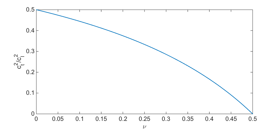
Figure 34: Wave speed ratio squared as a function of Poisson's ratio.
First we focus on the longitudinal direction of the Navier-equation without body forces (4.138), i.e., for component \( i=3 \). We note that the first term in (4.138) for \( i=3 \) is \( u_{i,kk}=u_{3,33} \) due to the assumption of a planar wave in Eq. (4.137). Similarly we note that \( u_{k,ki}=u_{3,33} \) for the same reason. Thus, the Navier-equation Eq. (4.138) in the longitudinal direction reduce to: $$ \begin{align} u_{3,33} \, \left (1+\frac{1}{1-2\nu} \right )&=\frac{\rho}{\mu} \, \ddot{u}_3 \tag{4.142} \end{align} $$ which may be presented in the form of a canonical wave equation: $$ \begin{equation} \partdd{u_3}{t} = c_l^2 \, \partdd{u_3}{x_3} \tag{4.143} \end{equation} $$ with \( c_l \) as defined in (4.139).
For the transverse directions, we use Greek indices to refer to the first two spatial directions only \( \alpha=(1,2) \). The Navier-equations (4.138) in the tranverse directions have a generic representation which also may be simplified due to the planar wave assumption in Eq. (4.137): $$ \begin{align} \underbrace{u_{\alpha,kk}}_{=u_{\alpha,33}}+\left (\frac{1}{1-2\nu} \right )\underbrace{u_{k,k\alpha}}_{=u_{k,3\alpha}=0}=\frac{\rho}{\mu} \, \ddot{u}_\alpha \tag{4.144} \end{align} $$ which is also a wave equation of the form as in (4.143): $$ \begin{equation} \partdd{u_\alpha}{t}=c^2_t \partdd{u_\alpha}{x_3} \tag{4.145} \end{equation} $$ with a wave speed given by (4.140). From (4.139) and (4.140) the ratio of the squared wave speeds may be expressed as: $$ \begin{equation} \frac{c_t^2}{c_l^2} = \frac{1-2\nu}{2\, (1-\nu)} \tag{4.146} \end{equation} $$ and further for \( c_l \) to be real we see that \( 0 < \nu < 0.5 \). The ratio of the squared wave speeds is plotted in Figure 34, and we see \( c_t < c_l \) for real \( c_l \).
Typically, steel have the material paramteters \( \nu=0.3 \), \( \eta=210 \, GPa \), and \( \rho=7.83\cdot 10^{3}\, kg/m^3 \) which corresponds to a transverse wave speed of \( c_t = 3212 \, m/s \), a longitudinal wave speed of \( c_l = 6009 \, m/s \), whereas the cylindrical bar assumption given by equation (4.141) gives \( c = 5179\, m/s \).
A longitudinal wave induces volume changes as \( \varepsilon_v = u_{3,3} = E_{33} \), and for that reason the wave is called a dilatational wave or a volumetric wave.
The stresses associated with the longitudinal waves are given by Hooke's law in equation (4.9): $$ \begin{equation} \tag{4.147} T_{33} = \frac{2 (1-\nu) \mu}{1-2\nu} \, u_{3,3}, \qquad \text{and} \qquad T_{11} = T_{22} = \frac{\nu}{1-\nu} \, T_{33} \end{equation} $$
The transverse waves are denoted isochoric, i.e., \( \varepsilon_v = 0 \), and for this reason also called dilatation free waves or equivoluminal waves. The corresonding stresses are found from Hooke's law as for the longitudinal waves: $$ \begin{equation} \tag{4.148} T_{13} = \mu u_{1,3}, \qquad \text{and} \qquad T_{23} = \mu u_{2,3} \end{equation} $$ From equation (4.148) we see that the transverse waves also has associated shear stresses on planes orthogonal to the direction of propagation, and for that reason they are also called shear waves.
Exercise 1: The generalized Hooke's law
a) Show that: $$ \begin{equation} E_{ij} = \frac{1+\nu}{\eta} \,T_{ij} - \frac{\nu}{\eta} \,T_{kk} \, \delta_{ij} \tag{4.149} \end{equation} $$
and $$ \begin{align} T_{ij} &=& \frac{\eta}{1+\nu} \, \left ( E_{ij} + \frac{\nu}{1-2\nu} \, E_{kk} \, \delta_{ij} \right ) \tag{4.150} \end{align} $$ are equivalent representations of the constitutive equation for an isotropic, linearly elastic material.
b) Derive Hooke's law for plane stress as given by the equations (4.36) and (4.37) from the general Hookean law represented by equations (4.7) and (4.9).
Exercise 2: Invariants
a) Show that that the time derivative of the right Green deformation tensor is given by: $$ \begin{equation} \dot{\boldsymbol{B}} = \boldsymbol{LB+BL}^T \tag{4.151} \end{equation} $$
Exercise 3: Shear modulus
Add a standard exercise for thin walled cylinder loaded with torsion from e.g. TKT 4123