Generating Mesh for 3D-DIC¶

Before you can run a 3D-DIC analysis, you need to generate two meshes (one for camera 1 and one for camera 2). The meshes shoud be identical, except for the nodal positions in the image.

It is assumed that you have two synchronized image sequence, one from camera 1 and one from camera 2.

Getting started¶

Open PreProcessor
Make sure that you see both views, i.e. that the “Camera Mode” dropdown list in the PreProcessor says “Both Cameras”
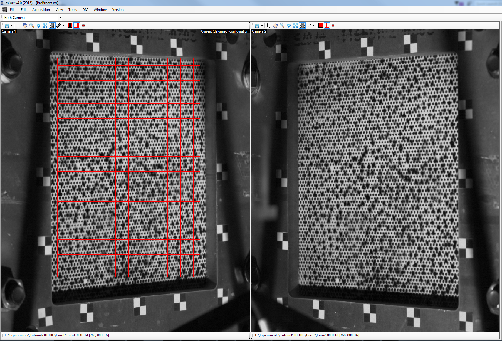
Load the first image in the image sequence for camera 1 in View 1 (LEFT) and the first image in the image sequence for camera 2 in View 2 (RIGHT). (see Image Panel on how to load images). Below you see an example of the PreProcessor where two initial images from two different cameras are loaded.

Generate mesh in View 1¶

We start by generating a mesh in View 1 (LEFT). This is identical as the procedure explained in Generating Mesh for 2D-DIC

Open Mesh Generation Tool. From Menubar: Tools -> Mesh -> Mesh Generation
In Mesh Generation Tool click “Generate structured Q4”
Specify the element size in the dialogbox that appears, or just accept default values
Click “OK”

An action called “Define polygon to make new Q4 mesh” appears in View1
Click in the image in View1 to define the polygon region of your new mesh
Click “V” in the action bar, or double-click on the last point of the polygon to accept

Hint

Hold “CTRL” to lock to horizontal or vertical axes when defining polygon region.

A mesh should be visible in View1

Modify mesh in View1 to fit the specimen¶

If you want to modify your mesh, you can open the Mesh Edit Tool
From the Menubar click Tools -> Mesh -> Mesh Edit
You can Translate, Scale and Rotate the mesh using this tool

A useful tool to position yor mesh in View1 is the “Modify Mesh Q4”, found in “Mesh Edit Tool”. If you click this button, you should see something like the image below.

Drag the four nodes to modify your mesh
The action are accepted by clicking the “V” in the action bar
Otherwise it can be cancelled by clicking the “X”

Extend mesh from View/Camera 1 to View/Camera 2¶

When you are happy with the way the mesh looks in View1, you are ready to extend the mesh to View2. This is where it differs from the procedure in Generating Mesh for 2D-DIC.

If you like, you can start by saving the mesh in View 1 (call the file something like “mesh_cam1.ecm”).

The process of extending the mesh from View1 to View 2 should result in a mesh in View2 which is identical to the mesh in View1, exept that the nodal positions (in the image) are different. The nodes should be located at the same “material points” of the specimen in both views. This process is done by a two-stage process:

First the mesh is extended to View2 and positioned roughly where it should be
Then the mesh in View2 is optimized using DIC to have the same position on the specimen as in View1. This optimization is also carried out in various steps as will be described later.

Open the Mesh Extender Tool from the menu bar: Tools -> Mesh -> Mesh Extender

You now have two options on how you extend the mesh from View1 to View 2.

Make a duplicte of the mesh in View1 and copy the mesh to View2. Then, you can modify the mesh manually to be situated similarly as in View1.
Make a set of reference points (corresponding locations in the images in View 1 and 2), and use these points to optimize the position of the mesh in View2.

Mesh Extend Option 1: Make duplicate and modify manually¶

Click “Extend mesh” in Mesh Extender Tool. The mesh in View1 is duplicated and added to View2

Open the Mesh Edit Tool In the menubar click Tools -> Mesh -> Mesh Edit
Make sure that the radiobutton at the top of Mesh Edit Tool is set to View2
Click on the “Modify Mesh Q4”
Drag the four nodes such that the mesh in View2 is situated similarly (on the specimen) as in View1
Press “V” to accept or “X” to cancel the action
You can also use “Translate Mesh”, “Rotate Mesh” and “Scale Mesh” in Mesh Edit Tool to position the mesh
Alternatively, “Modify Mesh Q8” can be used to obtain similar results

Mesh Extend Option 2: Extend mesh using reference points¶

Hint

Before you start this procedure it may be benefitial to hide the mesh present in View 1, so you can concentrate on the position of the reference points relative to the speckle pattern. (See image below on how to hide the mesh in a view)

In Mesh Extender Tool click “Add Point”. An action called “Click to define point” will be active in View1
Look at the images. Hopefully you will see some features on the specimen that are distiguishable in both views.
Click on such a point in View 1 and confirm the action (“V” in the action bar).
Now the “Click to define point” action should have become active in View 2. Click on the corresponding point in View 2 and confirm the action.
A new line should be added to the listbox in Mesh Extender Tool containing the positions of the two corresponding points you added.
Repeat this step to add multiple (preferable 4 or more) corresponding points between View 1 and View 2. It is preferable to select points with a high degree of separation.
When you now click “Extend Mesh” in Mesh Extender Tool a mesh is generated in View 2 which is a copy of View 1, but the nodal locations are optimized to fit the set of reference points you have added.

When you have generated the mesh in View 2, close the Mesh Extender Tool. The reference points shown in View 1 and 2 will dissappear and are no longer needed.

Optimizing the mesh in View 2¶

This is a very important step in order to obtain valid results from a 3D-DIC analysis. However, it can be a bit tricky...

It is assumed that you have followed the steps described above and have a mesh in View 1 and a mesh in View 2. The mesh in View 2 should have approximately the same position compared to the specimen as the mesh in View 1.

What we want to do now, is to optimize the mesh in View 2 using DIC, i.e., we will try to minimize the difference in grayvalues between the images in Views 1 and 2, by optimizing the nodal locations in the mesh in View 2. Depending on how successfully the rough positioning of the mesh in View 2 (as described above) was performed, this optimization can straight forward or challenging.

DIC is essentially a modified Newton-Raphson approach that searches for a global minima. If we are “far away” from the global minima when we start the correlation, DIC will converge to a local minima that may not be the correct global minima. DIC moves the nodes in an iterative process, and the maximum length a node can be moved is closely related to the spatial frequency of the speckle pattern in the area of the node. A speckle pattern with lots of local variations (high frequencies) will reduce the range of the nodal position updates in DIC. Thus, we can increase the range the nodes are allowed to be moved during this optimization by low-pass-filtering of the images, i.e. removing the high-frequency components of the speckle pattern in the image. This increases the chance of reaching the desired global minima, instead of some local minima that give false results.

Low-pass filtering of images are easily achieved using the Fast Fourier Transform (FFT) algorithm. FFT converts an image to a frequency domain. In the frequency domain we can mask out the frequencies we want to remove, before we go back to the spatial (image) domain using the inverse FFT. If we “mask out” the high frequencies when we are in the frequency domain, we end up with a low-pass filtered image.

This is basically a summary of the theory that we will use to optimize the mesh in View 2.

Open the DIC Tool (From the Menubar click Tools -> DIC)

Refering to the talk above, about local and global minima and low-pass-filtering of the images. It MAY BE... that you did an extremely good job (or just lucky) in the approximate positioning of the mesh in View 2. In any case, we will start by optimizing the mesh in View 2 without the use of FFT.

In the DIC Tool make sure that the “Use FFT” checkbox is un-checked.
In the dropdown list in DIC Tool choose “Full DIC” and press “Run DIC”

The DICCore.exe will open and carry out the correlation. When DICCore.exe closes, a new mesh will be loaded into View 2.

Note

If the DICCore.exe do not appear, and you get a dialogbox saying “Cannot start 2D-DIC process”, go to menubar: Edit -> Settings, choose the “Analysis” tab. The path labelled “DIC Core Folder” should point to the location of the “DICCore.exe” file. This is normally located in a folder named “core”. Browse and find this folder. Click “Apply” to close the “Settings Window”. Now you can try running the DIC as described above.

Does the optimized mesh in View 2 look good (or better than before)?

If YES, run the “Full DIC” a couple more times before you save the mesh :ref:saving_mesh. Ideally the number of iterations should not reach maximum in the console program.
If NO, you need to keep on reading this section.

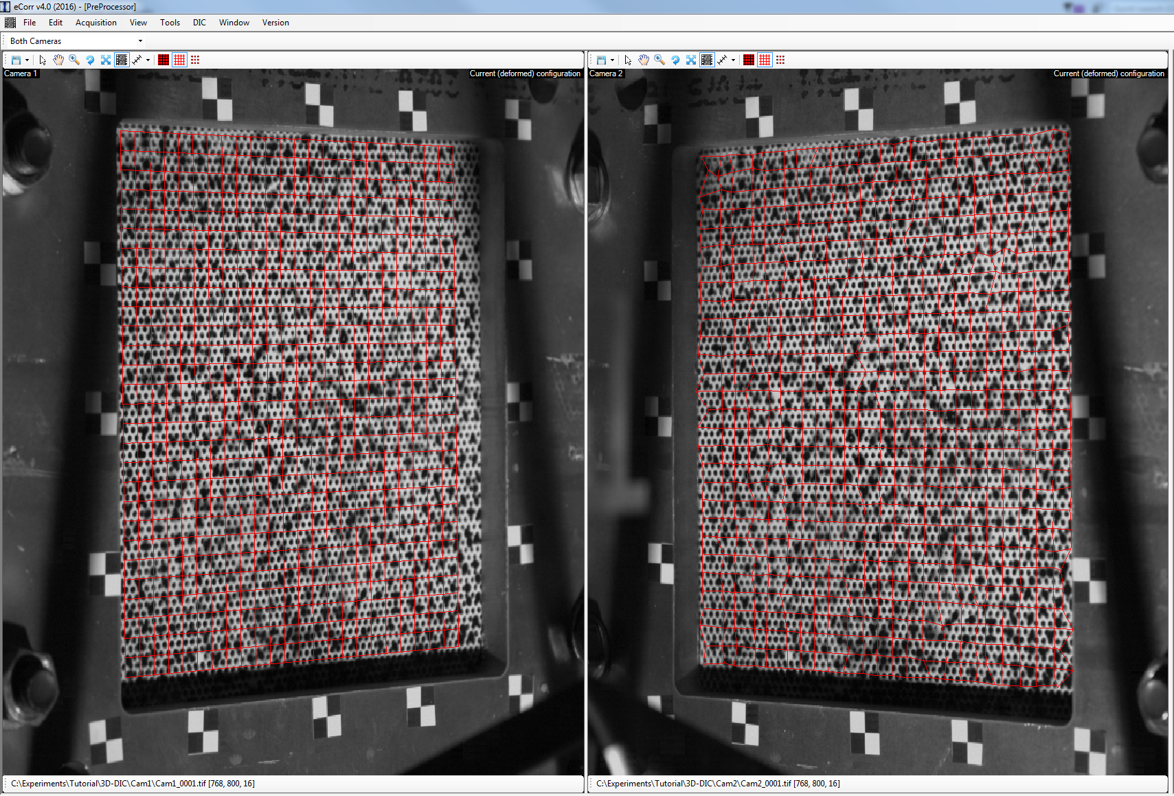
Below is an exable of a non-successfull DIC between the two views. Some of the elements in themesh in View2 is distorted due to poor correlation.

Multiscale coarse-search optimization¶

As explained above, the “Full DIC” approach may not succeed because the starting point (nodal locations) are too far away from the global minima that is searched for.

The strategy here is to apply a two-fold procedure where the image is low-pass filtered (using FFT) at the same time as the degrees-of-freedom (DOFs) in the DIC procedure is reduced.

The two parts of this strategy is explained in the following sub-sections.

FFT Filtering¶

At the top of the DIC Tool you see the options for FFT filtering of the image:

If you check the “Use FFT” checkbox, the FFT will be initiated for the current images in View 1 and 2. If you type in a “Mask size” and press “Enter”, the images in View 1 and 2 will be filtered. Below you will see how an image will look when you apply different mask sizes. The Range of the mask is (1 - 500).

A low mask value (close to 0) will result in a strong low-pass filter, removing most of the frequencies except the frequencies with the largest wave-lengths.

A high mask value (close to 500) will result in a week low-pass filter, resulting in an image that is very close to the original image.

Below are some examples of images filtered with varying mask sizes.

Raw image

Mask Size = 200

Mask Size = 100

Mask Size = 50

Mask Size = 10

Reducing DIC degrees of freedom¶

At the bottom of the DIC Tool you see the options for reducing the degrees-of-freedom in the correlation between the views:

The options are:

Rigid body: (2 DOF) Here, there is only two degrees-of-freedom in the entire mesh. Its a rigid body translation in the horizontal and vertical directions.
Super Q4: (8 DOF) A virtual Q4 element is generated covering the entire mesh. The nodal positions in the mesh is controled by this large element.
Super Q8: (16 DOF) A virtual Q8 element is generated covering the entire mesh. The nodal positions in the mesh is controled by this large element.
Super Multiple: Similar as “Super Q4” and “Super Q8”, but here multiple super-elements can cover the entire mesh.
Propagating Subset: Not yet implemented!
Full DIC: A full DIC of the entire mesh. The degrees of freedom is equal to twice the number of nodes in the mesh.

Combining FFT filtering of image and reduced DOFs in DIC¶

If you have not already done so, in the DIC Tool check the “Use FFT” checkbox.

The multi-scale coarse search optimization is usually performed in multiple steps, which are controlled manually.

Type in the choosen “Mask size” (a value between 1 and 500).
Select the type of correlation (degrees of freedom).
Press the “Run DIC” button in the DIC Tool.

When the correlation is completed, the mesh in View2 should be updated.

Visually evaluate whether the correlation was successfull or not (if the mesh is closer to the correct position)

Every time you run a correlation the mesh in the view is updated. However, the software keeps all the meshes in memory. If you open the Mesh List Tool (From menubar: Tools -> Mesh -> Mesh List), you can go back and see how the mesh is altered at each step. You can also choose an older mesh to be the starting point of the next correlation (if the latest correlation didn’t succeed).

Note that the mesh currently visible in View2 is the starting point for the correlation when you press “Run DIC” in the DIC Tool.

The choice of mask sizes and correlation types (degrees-of-freedom) may be difficult to make, and a general approach is even more difficult to state. However, this coarse-search optimization is a relative powerful tool, and there may be multple paths that lead to the correct end-point.

As a default procedure, you can try:

Mask size 60, Rigid Body
Mask size 80, Rigid Body
Mask size 100, Super Q4
Mask size 150, Super Q8
Mask size 250, Super Q8

Evaluate between each step wheter the step is successfull or if you need to alter the mask size, or if you need to run the optimization multiple times for a single step.

As a final step, uncheck the “Use FFT” checkbox (the current image is now the original image), choose “Full DIC” and press “Run DIC”. The resulting elements in the mesh should NOT be distorted. If som elements are distorted you may deactivate them using the Mesh Edit Tool, or you can go back to an earlier mesh using the Mesh List Tool and try a different path of mask sizes and correlation types.

Note

It may be a good idea to run the final “Full DIC” at the original image a couple of times. In the console window you can see wether the correlation reaches maximum iterations or if the criteria is reached. Ideally the criteria should be reached, but in some cases it is not possible.

Saving the meshes¶

You need to save the meshes, both in View 1 and in View 2 as mesh files (*.ecm). The “Save mesh” option is found by pressing the floppy icon at the top-left corner of each view.

When you save the mesh in View 2, a dialogbox will appear like this:

This is because the mesh has non-zero nodal displacements. All correlation steps carried out to optimize the nodal locations of the mesh in View 2, has given the mesh non-zero nodal displacements. A mesh used as starting point for a 3D-DIC analysis should have zero nodal displacements.

Accept the default settings (Save the mesh as reference mesh (no nodal displacements), and add all nodal displacements to the initial nodal locations), and press “OK”.

You have now generated two meshes (one for Camera 1 and one for Camera 2). The meshes are identical except for different nodal locations in image coordinates. The nodal locations on the specimen (in target space) however, should correspond for the two meshes.

You may now close the PreProcessor and proceed with the generation of input file for the 3D-DIC analysis.