Study Results for 3D-DIC
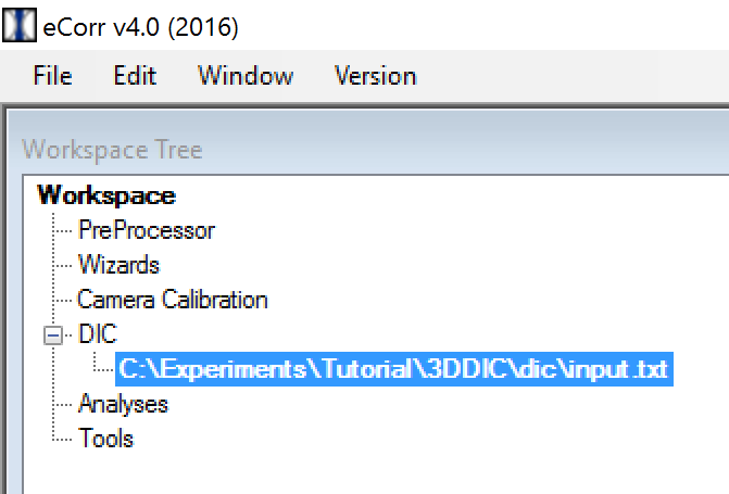
If you have just run a DIC analysis (as described in Make and Run 3D-DIC Input File), you will see the DIC input file under the DIC node in the Workspace Tree.
Otherwise, you can open the input file by right-clicking the DIC node and click “Load Input File...” in the context menu.
It is possible to visualize the data both in an image view (Results View (Image)) and in a 3D view (Results View (3D)).
Results View (Image)
To open the Results View (Image), right-click on the input file in the Workspace Tree and choose “Results View (image)”.

The Results View (Image) will be shown like this:

The list at the right side of the Results View (Image) shows all image indices defined in the input file. Click on a specific index to view the corresponding pair of images for Camera 1 and Camera 2.
Check and Modify the Target Coordinate System
The target (three-dimensional) coordinate system used in the 3D-DIC analysis is basically a result of the camera calibration. Thus, the plate seen in the images from camera 1 and camera 2 may have an arbitrarly rotation and translation compared to this coordinate system.
An indication of this can be given by visualizing the location in Z [mm] as a field map.
- Open the Field Map Tool (from menubar: Tools -> Field Maps).
- In the Field Map Tool, expand the node called “Location”
- Right-click on “Z [mm]” under the “Location” node and choose “Set as Field Map” in the context menu that appears.
The field map illustrating the Z location, may look like this:
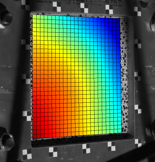
It is clear that the plate is not situated in the XY plane. If we want the plate to be situated in the XY-plane and the Z coordinate representing the out-of-plane direction, we need to correct the data by applying a rigid-body trasnformation of the data.
- Open the Configuration Manager (from menubar: Tools -> Configuration Manager).
In the Configuration Manager you will se 6 textboxes representing 3 angles of rotation and 3 offsets in position. For a new input file, these values should be zero. The values represent the rigid-body transformation correction of the data.
- Click the “Optimize initial plane” in the Configuration Manager
Some of the 6 rigid-body correction values should be updated to non-zero values.
In View1 (if you haven’t cleared the field map from the previous step), you should see the updated Z-location field map. Now, the z-location field map illustartes the topography of the plate.
In the example data, the field map looks like this:
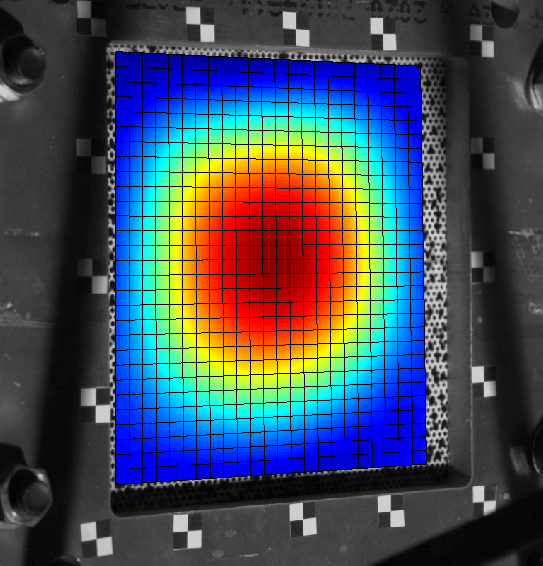
The z-location is no longer dominated by a rotation of the plate compared to the XY-plane, but of an initial curvature of the plate. In this case the maximum deflection of the 400x400mm2 plate is approximately 2mm. The reason for this deflection will not be discussed here, however, it is in general important at this point to make sure that such deflections are physical and not a result of a poor camera calibration.
The rigid-body correction constants are automatically saved for this particular input file when the Configuration Manager is closed. When you open the input file at a later point, these rigid-body correction values will also be loaded.
Visualization, Plotting and Exporting Data
Similarly as for a 2D-DIC analysis, you can visualize field maps using the Field Map Tool, plot data in graphs using the Graph Tool and export data to text files using ../components/gui/tools/filewrite (See :doc:../2ddic/studyresults2d` for details on this).
The main difference between a 2D and a 3D-DIC analysis here, is that you have more data available in a 3D-DIC analysis. This is illustarted in this figure of the Field Map Tool:

Here you have a node called “2D (Cam1)”. This is all DIC data for a 2D-DIC analysis of the images from camera 1. If you check the “View 2” radio button at the top of the Field Map Tool, this node will change name to “2D (Cam2)” and contain all data from a 2D-DIC analysis of the images from camera 2. The “3D” node, on the other hand, contains the available 3D data (displacements, strains, etc...).
Generating videos
Videos of the image series with various field maps may be generated using the Video Generation Tool (from menubar: Tools -> Video Generation). (See Video Generation Tool for details on how a video can be generated)
Results View (3D)
To open the Results View (3D), right-click on the input file in the Workspace Tree and choose “Results View (3D)”.

The Results View (3D) will be shown like this:

If you get an error when trying to open the Results View (3D), the reason may be that you don’t have the needed DirectX version (DX9) installed on your computer. The DX9 redistributables may be found here:
or here:
Generating videos
Videos of the 3D models with various field maps may be generated using the Video Generation Tool (from menubar: Tools -> Video Generation). (See Video Generation Tool for details on how a video can be generated)