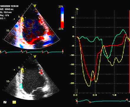
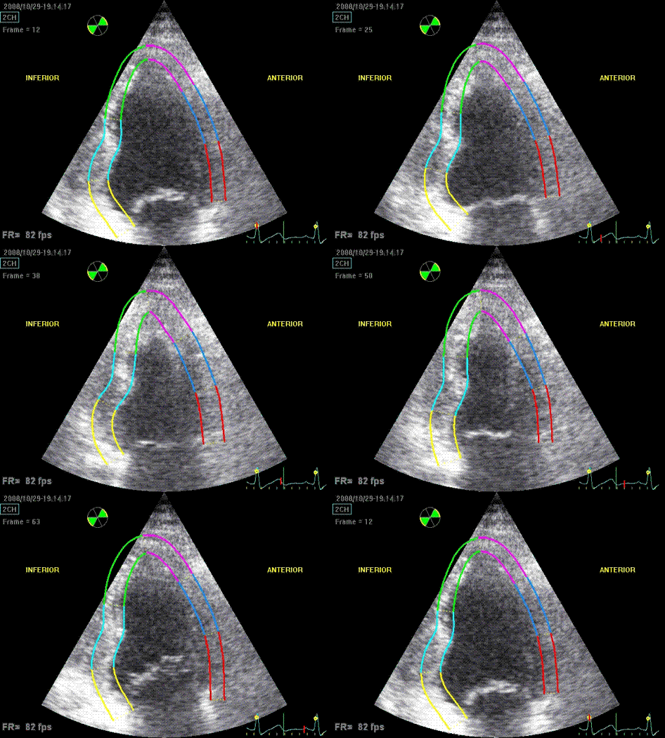
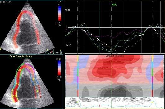
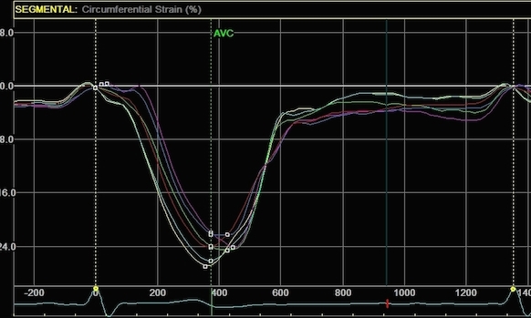
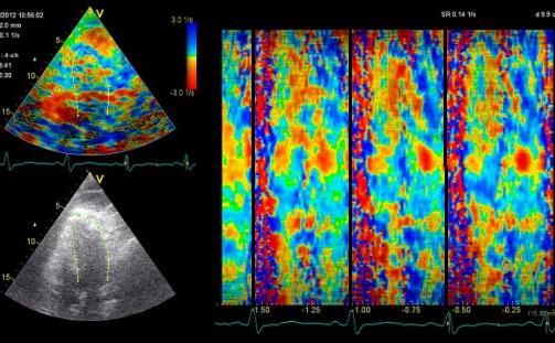
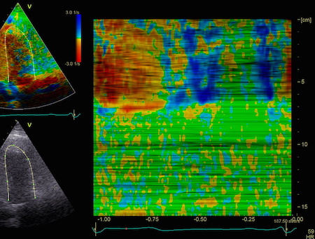
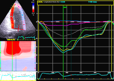
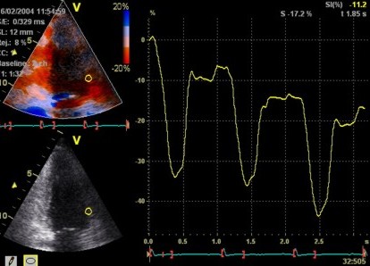
Brown skua hunting gentoo chicks. Danco Island, Antarctica.

Problems and pitfalls

Limitations and artefacts related to strain rate imaging

The page is part of the website on Strain rate imaging
by
Asbjørn Støylen, Dr. med.

Goshawk with prey. My garden.

This section updated: June 2016


Basically, irrespectively of method, the fundamental indices of motion (velocity and displacement) and of deformation (strain rate and strain) are the same. Also, the display of the indices can be used across some of the methods for acquiring them.

The fundamental limitations of ultrasound apply. The poorer the image quality, the less useful are any of the methods:
Garbage in - garbage out.

In addition, there are specific problems that arise from the specific application of the basic methods to deformation measurement, as well as how the methods are dealt with, which creates new pitfalls. The present section have been re edited, so the main headings are now the problems and limitations themselves, and the effect on each of the different methods are described under those headings.

There are four sets of limitations:

However, in dealing with the noise problem, new problems may be introduced, specific to the smoothing methods used. This is in general more problematic in some speckle tracking methods than in tissue Doppler.
In addition, there is the point of experience dependency. This has been very clearly demonstrated in WMS in stress echo, but all methods have a learning curve, so experience dependency is a feature of all methods. And in strain rate imaging, much of the experience is in
However, the main point is that areas with poor data quality should not be analysed by any method. Garbage in, garbage out!


Section Index

Back to website index

Limitations of WMS

All limitations due to image quality are pertinent also to wall motion score, although B-mode is one of the most robust method. Poor endocardial definition, however, especially due to drop outs, will be especiallly deleterious. The use of contrast, however, may improve this substantially. Using contrast improves the LV delineation, but on the other hand, this will shift focus somewhat towards endocardial excursion, instead of wall thickening, increasing the susceptibility for tethering, as tethering may pull passive segments both inwards and in the apical direction. This limitation is much less pronounced with strain rate imaging, as the methods themselves subtract motion due to tethering.

In WMS, Especially in stress echo, it has been shown that reproducible wall motion score grading is experience dependent, beyond general echocardiography experience (101). Thus, the exact assessment of regional reduced function may be experience dependent.

Assessment of wall thickening may be difficult, especially in the basal segment, where there is a large component of longitudinal motion, even in akinetic segments. Subtracting that may lead to overestimation of wall thickening.

Looking at the ventricle in cross sectional slices, the thickening may be more evident. However, parasternal windows may be limited, but with 3D-dimensional ultrasund, cross sectional slices can be reconstructed either from apical or parasternal windows. Then, the confusing long axis motion is eliminated from the image. When the cross sectional plane also is made to track the tissue, the effects of out of plane motion can be eliminated from the cross sectional slices.

Fundamental limitations of ultrasound.

Thus, for a start the fundamental limitations of ultrasound have to be known. The mechanisms for these are discussed in the basic ultrasound and Doppler sections, so in this section we take the discussion further into the consequences for each specific method.


Out of plane motion in parasternal images


The base of the heart moves about 1.5 cm towards the stationary apex during systole. This means that even at the level of the papillary muscles, closer to the mid ventricle, the motion will be 0.7 to 1.0 cm (the imaging plane / line) is often placed a little basal to the equator.


Parasternal long axis image. The longitudinal motion of the basis is evident.
The yellow line crosses the ventricle near the middle in end diastole, but much closer to the base in systole, transecting a different part of the myocardium.


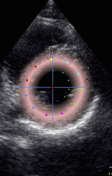
Parasternal short axis image. Even if it looks stationary, the short axis plane is moving in and out of the imaging plane, so there are different parts of the ventricle being images in systole and diastole
Which is evident from these still frames. In diastole (top), the ventricle is imaged at the level of the insertion of the papilary muscles and the moderator band, in systole 8 bottom, the base of the heart has moved so the ventricle now is imaged at the level of the chorda tendineae, while the papillary muscles and imoderator band has mpoved apically, out of the imaging plane.

This, of course affects the M-mode measurements as shown below:


However, as the imaging plane contains different parts of the LV in systole and diastole, speckle tracking in short axis views actually don't see the same acoustic markers in systole and diastole, so it's not real speckle tracing in the sense that the same speckles are tracked throughout the heart cycle, as discussed below.


Foreshortening


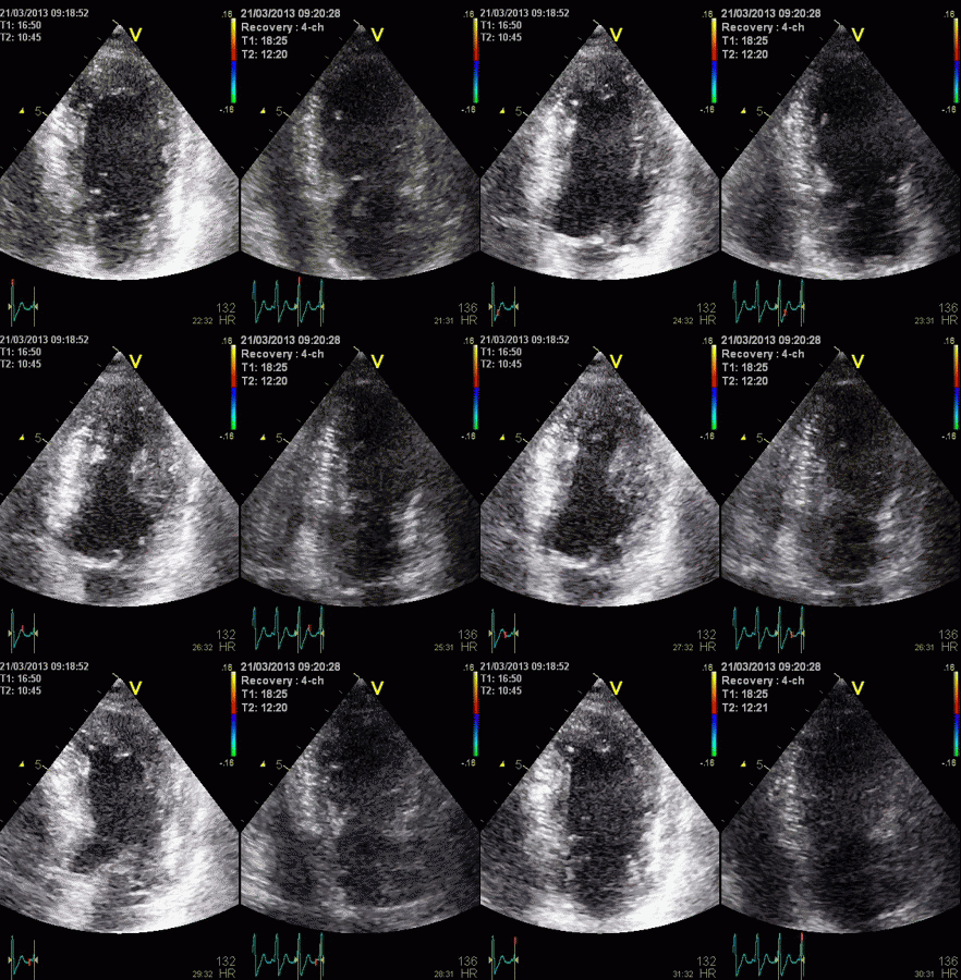
Foreshortening ilooks better i four chamber view, but rotating the probe shows the aopex to be out of sector.
In the foreshortened image to the left, the dyskinetic area anteroapically is not visible.


will cause

Shadows will either cause drop outs, or reduce image quality over all due to reduced effective aperture as discussed in the basic ultrasound section.

The main point of shadows is that without any imagem there is nothing to track neither by tissue Doppler nor by speckle tracking.


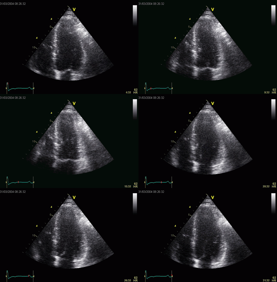
Drop out affecting speckle tracking. The application cannot track where there are no tissue data, in this case in the anterior wall and the application doesn't track (the markings don't move). The inferior wall seems to track normally. (Which is untrue, there is an inferior infarct)
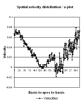
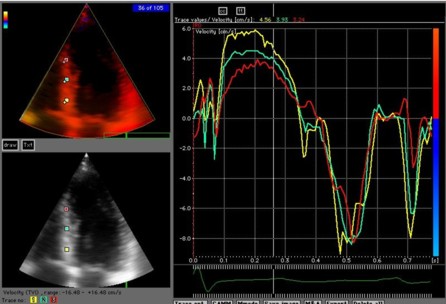
V-plot in a two-chamber view, showing fairly normal velocities in the inferior wall (except for a small reverberation). The anterior wall shows a shadow, with low velocities. Thus, the slope of the velocities is low as well, and thus a low strain rate.

However, due to the specific algorithm of the velocity gradient method, there are some specific pitfalls as well, leading to overestimation of the strain rate below the drop out:


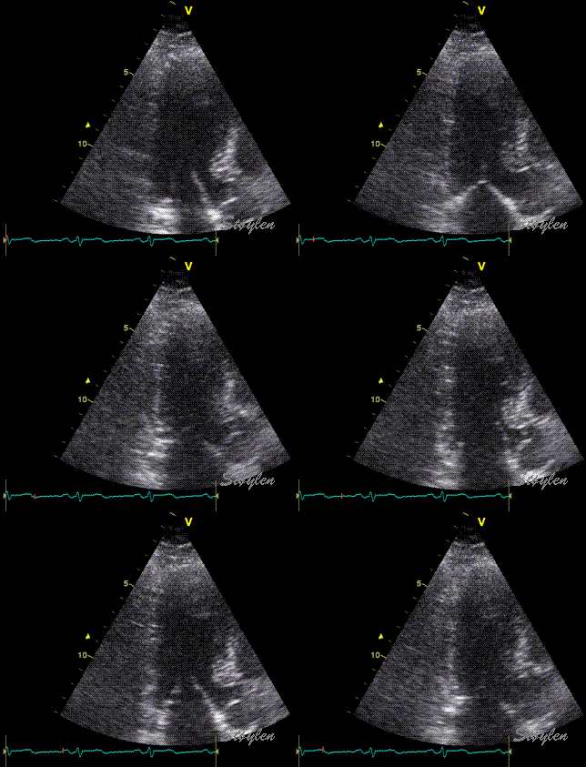
Drop out in the anterior wall. In this area there are no B-mode data, indicating that there are no velocity data either (although this may not always be the case).
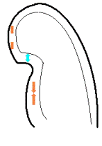
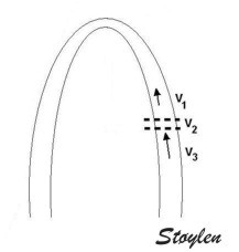
Schematic figure corresponding to the loop to the left. In this case there are no data in the drop out, resulting in zero velocity, i.e.  v1 = 0.
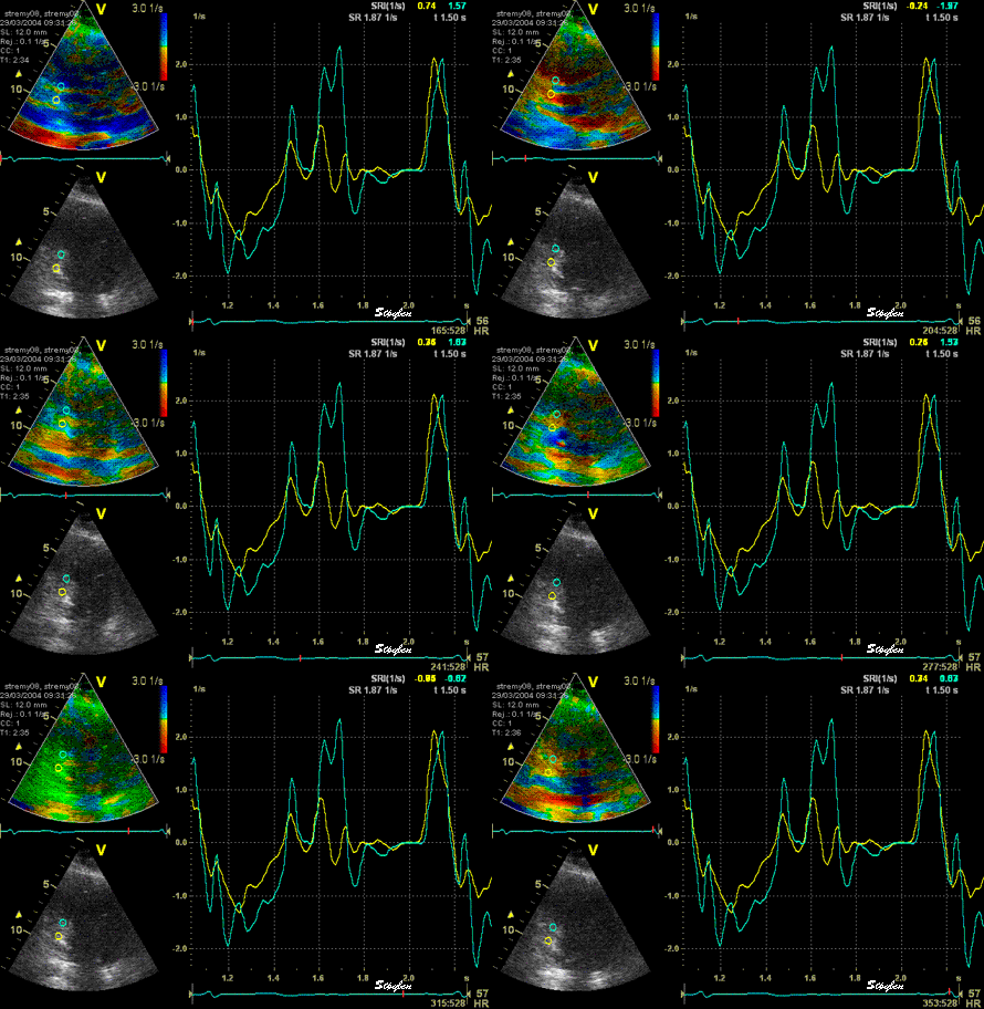
As is evident from the traces, the velocity in the drop out area (cyan curve) is zero. Below the drop out, the velocity curve is normal.


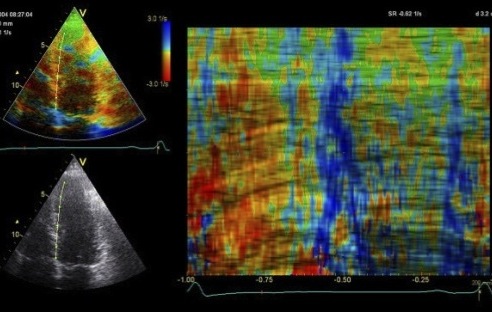
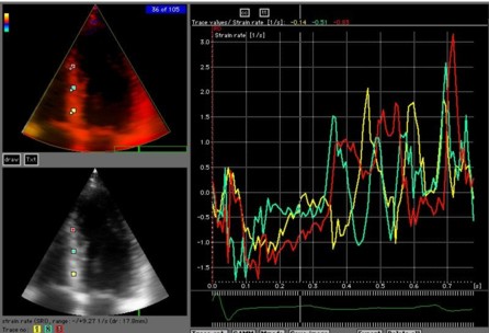
The effect on strain rate, however, may seem a little paradoxical. Below the drop out, there are much higher absolute strain rates. This can be explained by the subtraction algorithm, (although a little simplified), as SR = (V1 - V2) / L,  as V1 = zero, this will result in SR = - V2, i.e. the strain rate curve becomes an inverted velocity curve.  Thus, the absolute values will be much higher that the real strain rate.  This can be seen in the transitional zone where the strain length crosses the border between the drop out and the normal  area (cyan curve). Observe how the curve looks almost the same as the normal velocity curve above (yellow velocity curve).  The more basal measurement, with all of the strain length within normal data, shows normal values (yellow curve).  The curved M-mode shows the distribution of the effects. In the apex (1), there are no data for strain rate, showing no deformation. (the whole strain length is within the drop out.  In the midwall (2), there are exaggerated strain rate values, shown by the colour intensity (red) equivalent to the cyan curve to the left. In the base (3) there are normal strain rate values (orange) equivalent to the yellow curve to the left.


Reverberations (clutter)

will result in insufficient tracking in both tissue Doppler and speckle tracking. As tissue Doppler is done in the fundamental mode to avoid aliasing, while B-mode images are acquired in the harmonic mode, there may be some difference to the susceptibility to reverberation noise. However, much of the apparent lower susceptibility of speckle tracking applications are due to smoothing algorithms, that results in apparent tracking due to interpolation of data from other regions. This means that the tracking in areas of clutter is not real, only apparent, and the same smoothing may mask regional dysfunction to some degree.


Discrete stationary reverberations, are areas of discrete stationary echoes due to an ultrasound pulse bouncing between the probe and some structure in the patient, as described here.

Stationary reverberations

In stationary reverberations, the effect on strain rate imaging is that both areas above and below the reverberations are affected, especially in speckle tracking.


Stationary reverberations shown in B-mode, the mechanism is explained in the ultrasound section. Stationary echoes are called clutter.

Reverberations in speckle tracking

In speckle tracking, the stationary reverberations will result in stationary speckles, and thus an area that is not tracked.

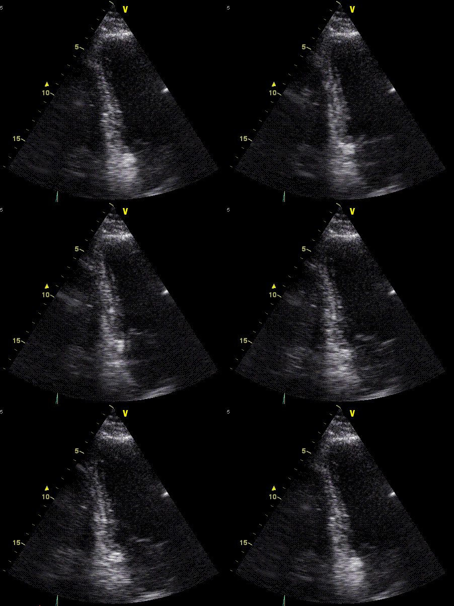
Reverberation in the lateral wall affecting speckle tracking (same example as above. As is visually evident, the application does not track across the reverberation, thus the two segments apical to the reverberations are seen as akinetic, the basal as hyperkinetic. All shortening is seen in the basal segment. In this case, the smoothing is seen to spread the effect of the reverberation out across two segments apical to the reverberation.

Thus, this will result in erroneous values both above and below the reverberation as seen above, actually affecting all three segments of the wall.

Reverberations in segmental strain


If the algorithm does not track one kernel correctly, the strain values will be wrong for the segments on both sides of the kernel. This is evident in areas of drop outs or reverberations as illustrated schematically below.


Effect of a reverberation on the border between the apical lateral and the midwall lateral segment. A kernel  in this area will not track, as illustrated by the arrow.  The next border between the basal and midwall segment moves normally, leading to an exaggerated shortening of the midwall segment, while the basal segment shortens normally. (The segmental strain in the apex is the difference between the apical motion (zero) and  the apparent motion ( near zero) in the reverberation, the midwall strain is the difference between the apparent motion ( near zero) in the reverberation and the (normal) motion of the border below.) This is evident by the curves (compare to the average curve: The apical curve shows little strain, the midwall curve shows far more than the wall average, and the basal shows average strain).  Compare with the image above. Image courtesy of H Dahlen.
The kernel is in a reverberation in the lateral wall, and will not track. In this example the reverberation is in the border between the basal and midwall segment. the shortening of the basal segment is exaggerated, and the shortening of the midwall segment is reduced.

Thus, one kernel tracking poorly will then lead to two segments being discarded, giving a high discard percentage. This was seen in the HUNT study with automated analysis, we consider this an advantage of the study, leading to little contamination of the data by artifacts, thus ensuring the data to be "clean". However, it is a disadvantage of the method, leading to a lower feasibility. However, in clinical studies, the feasibility was around 80%, and in addition showin added diagnostic value to B-mode (128). But basically a high discard rate ensures higher quality of the studies.

However, in the segmental method, the reverberation can be avoided by replacing the kernel:


The kernel is in a reverberation in the lateral wall, and will not track, thus both the segment below and above the reverberation will show artefacts.
Adjusting the position of the kernel manually, allows speckle tracking despite the reverberation, if the kernel remains outside the reverberation during the whole heart cycle.

Thus offering a little more versatility than the above method.

Reverberations in tissue Doppler


As discussed under Tissue Doppler, the presence of clutter noise(reverberations) affects autocorrelation derived tissue velocities, but peak values by spectral Doppler are still visible and renders clutter more irrelevant. However, in autocorrelation, this wrecks havoc with the ordered sequence of velocity curves that is necessary to derive strain rate:


Tissue Doppler in the presence of heavy clutter. Left, autocorrelation, showing low velocities, but especially in the middle sample volume than is within the heaviest reverberation, where peak S' is 1 cm/s, and then increasing to near 2 cm/s closer to the apex. however, the presence of clutter all over results in all measurements being underestimated as stationary echoes are included in the mean velocities. Right the spectral tissue Doppler from the same sites, acquired sequentially by pw tissue Doppler. the peak values are unaffected of the heavy clutter band around zero.

In this case, the subtraction algorithm leads to quite different effects.


Explanatory diagram. v1 and v3 have normal velocity measurements, while v2 is zero. This results in all strain rates measured in the segment above the reverberation will show normal strain rate. A sample across the reverberation, resulting in SR = v1 - v2, will give a positive strain rate, while a sample volume across the strain rate below, SR = v2 - v3 will give a negative strain rate, but over estimating the magnitude
Same example as above. The result in tissue Doppler is that the reverberation shows up as a stationary area of inverted colour on the cine loop. This corresponds to a horizontal band in the M-mode, showing sharply in the strain rate image. However, there is also accentuated strainrate below the reverberation showing up as a deep red colour.


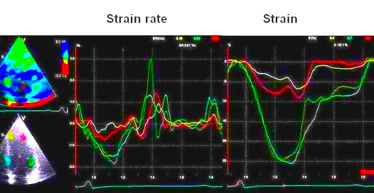
Above the reverberation, where all of the strain length is in normal signals, the strain rate is normal (orange in systole, blue in diastole. In the area where the V1 end of the strain length is in the normal area, and the V2 end is in the reverberation, and thus = 0,  the strain rate will be SR = (V1 -V2) / L = V1 / L. This is seen in the yellow curves, looking like normal velocity and displacement curves. As systolic shortening is negative, while velocity and displacement are positive, there is apparent dyskinesia in this area.  This area shows inverted strain rate in the M-mode to the left.  Below the reverberation, where the apical end of the strain length is in the reverberation, and the basal end is in the normal velocity field, the effect will be SR = (V2 -V3) / L = -V3 / L as shown by the deeper colour (red) and the cyan strain rate curve, equivalent to the inverted velocity curve shown in the drop out artifact. Thus we have apparent hyperkinesia.  Finally, the red and green curves are both from the transitional zone, being interpolations between the other artifacts. The green would be apparent initial dyskinesia, while the red is apparently normal. However, as the whole area has data quality arising from artifacts, NONE of the curves should be used, lest there be biased post processing.  The whole area should be discarded.

But this means that as tissue Doppler measures are independent of measurements in the other segments, this is the only method where the whole area above the reverberation is unaffected.


Strain rate 3D mapping of normal ventricle showing a reverberation in the septum
Showing up as blue colour during ejection, and increased red colour basally to the reverberation
and red colur during diastole, with increased blue colour basally.

Basically clutter is stationary echoes resulting in zero velocities as decribed more in detail in the basic ultrasound section. Thus, cutter is basically systematic noise, not random. However, in colour tissue Doppler clutter will also lead to increase in random noise. This is again due to the autocorrelation algorithm. The velocity estimate in each pixel will be an average of the amount of clutter and of moving echoes. The final velocity estimate will vary according to the relative amplitude of the clutter and the moving echo (weighted) (284), and this varies according to the speckle pattern as described here. Thus, in areas with much clutter, the velocity variations are larger than in high quality recordings:

Image with reasonable quality showing a moderate amount of random noise
Image with reverberations. The average velocity values are lower, but in additions the variation of the velocity estimates from pixel to pixel is much higher.

Thus, with an increase in random noise as well, there will be even more variability of velocity estimates and even more in strain rate estimates.


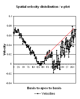
Two chamber V-plot from a patient with reverberations in the inferior wa... The figure illustrates the variability of the velocity curves taken from different parts of the wall. There is also a drop out in the anterior wall, mimicking an anterior infarct. After (247)


Thus, The V-plot might be more robust for clutter that strain rate curves, as the increased variability is fairly visible (247). This is due to the fact that there is a high variability in velocities from pixel to pixel, so the slope on top of the highest  velocities may be seen to reflect strain rate:

The slope can be discerned despite heavy reverberation noise.

(However, the main problem of V-plot in colour Doppler is the drop outs/incoherent reverberations , as an infarct and a drop out may look completely similar in the V-plot from colour tissue Doppler.. )


A: Fairly good quality normal 4-chamber view, showing the normal V.
B: 2-chamber view from healthy subject, showing an inferior reverberation (note, the true slope can still be discerned) and an anterior drop out.
C: 2-chamber view with moderate clutter in the inferior wall and an anterior wall infarct.
D: 2-chamber view with inferior infarct in the basal part (see the suddenly decreased slope) and an anterior drop out.
(Image courtesy of E. Sagberg.)

It is evident that there is no way by the V-plot alone to reliably see the difference between a drop out and an infarct or clutter.

Retrospective spectral tissue Doppler, acquired as IQ data from ultrafast Doppler imaging, however, will be able to render clutter at least, but also drop outs to some degree, irrelevant. With simultaneous spectral Doppler data over the whole field, V-plots can be generated as spectral V-plots.


Spectral Doppler V-plot from apical long axis. There is substantial clutter in the inferiolateral wall. This is rendered irrelevant by using spectral Doppler.
There is drop out in the anterior wall. This will to a certain degree affect the spectral Doppler, but by gaining up in post processing, it is possible to see that there is signal in what appears a "through"in the wall, indicating a normal slope. The autocorrelation V-plot is included for comparison, again showing how both clutter and drop outs leads to under estimation.


On the other hand, the problem of reverberations are greater in tissue Doppler, as this is done in fundamental, and not harmonic mode. Harmonic imaging is not feasible in tissue velocity imaging, due to the low tissue velocities. This results in a low Nykvist limit at harmonic frequencies, resulting in aliasing in tissue Doppler at ordinary tissue velocities as shown here. Although strain rate would unwrap most of the aliasing, this would mean that separate recordings would have to be made for velocity (fundamental) and deformation (harmonic) imaging, instead of deformation being post processed from velocity recordings. However, it might solve some of the reverberation problems.


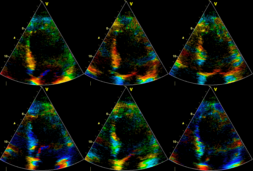
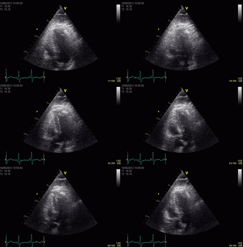
Image with shadowy reverberations. The 2D image doesn't seem too bad, as the movement of the wall is fairly well visualised.
Strain rate in the same image.  Shadowy reverberations are better visualised in this image.
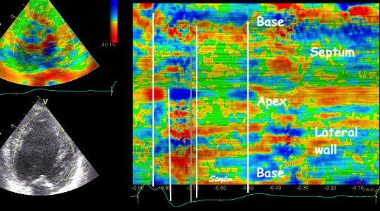
Curved M-mode from the lateral wall. Apex on top, base at the bottom. The S, e and a phases can be seen, but that is about all the information that can be extracted.

Thus, colour M-mode shows the data quality, especially in the M-mode.

Colour M-mode gives timing information even in in poor images

Heavy reverberations will show up, and the Colour M-mode will tell about timing parameters, and say if the quality is good enough to extract  deformation curves.

However, the problem of reverberation noise is not so great in using colour M-mode. The information is qualitative rather than quantitative, and the reverberations are fairly easily identified as horizontal bands of reversed colour. But the colour M-mode also gives timing information, and this information is quantitative.


The reverberation is easily identified in the M-mode, and the timing of the phases of the heart cycle is evident despite the reverberation. All the phases of the cardiac cycle can be seen and the timing seems normal. In this case there is left bundle branch block, with reverberations in the lateral wall. Still the septal flash with lateral stretch, the lateral wall shorteining with early and late septal stretch and the septal post systolic shortening (recoil) can be seen. The image can guide the placement of ROIs, but the information should still be used only qualitatively.

Both delayed onset and post systolic shortening are indicative of reduced regional function, and may be identified or excluded even in images of poor quality:

Any kind of stationary echo noise is termed clutter.  Due to the autocorrelation algorithm, the velocity measurements may be averaged into the velocity estimate, resulting in too low values. this means that the timing information, which is visualised through colur M-mode may be visible, while peak values will be incorrect.


Stress acquisition at peak stress in a patient with extremely poor image quality due to seriously thickened pericardium after a previous CABG, plus emphysema. The lateral wall cannot be evaluated at all.
Curved M-mode from the same view in a TDI acquisition at peak stress. Even if the signal is noisy, the onset of shortening can be delieated (black lines), thus showing symmetric onset in both walls.

The advantage of wall motion by colour M-mode is it's robustness, especially in relation to reverberation noise. Still, the fundamental limitations of ultrasound as well as specific for image quality applies, poor image quality will affect the interpretations. Especially drop outs may illude as akinesia.


Non coherent clutter:

If clutter is non coherent, and extensive, of course no method will measure any deformation at all:


Shadowy reverberations covering the anterior wall in this 2-chamber image. We se a "fog" of structures covering the anterior wall. The structures are stationary. This is not distinct reverberations shadows, but incoherent clutter.


Same examination as above in TDI. CAMM drawn from inferor base through apex to anterior base. The whole of the anterior wall shows green area of no strain, spots of yellow and blue are noise spikes.
Same examination as above in TDI. Again, the whole of the anterior wall shows no strain (magenta, blue and red curves, peak strain values < - 2.5%).

This is also evident from the V-plots shown above:

Lateral resolution


Lateral resolution in speckle tracking


This is dependent on both line width (being dependent again on frequency and focus depth), and line density (being dependent on frame rate and sector width). In addition, there has to be adequate alignment of the ultrasound beam, as angle deviation will reduce the number of lines within the wall in the far field. This is true for speckle tracking as well as tissue Doppler. Finally, focusing of the beams will result in different lateral resolution at different depths.


Speckle tracking has the advantage of a higher line density of B-mode, at the cost of a lower temporal resolution.  The very low lateral resolution used in tissue Doppler in order to achieve a high frame rate, results in a low line density, and in practice limits the measurement in the beams in the longitudinal (and tangential - for circimferential measures) direction to the entire wall thickness, for a standard set up.


A: Beam width. Speckles (true speckles: black) are smeared out across the whole beam width ( Apparent speckles dark grey, top). This means that with this beam width the speckles from to different layers cannot be differentiated, and layer specific motion cannot be tracked.
B: Line density. Only the lines in the ultrasound beams (black) are detected, and can be tracked, beams between lines are not detected or tracked.and differential mtion of the two speckles cannot be tracked. The spaces between lines cannot be seen doe to image lateral smoothing.
C:  Divergence of lines in the depth due to the sector image will both increase beam width and decrease line density in the far field. this may result in the line density and width being adequate (in this example for two layer tracking) in the near field, but inadequate in the far field, situation there being analoguous to A.
D:  Focussing. The beams being focussed at a certain depth mau mean that line density may be inadequate at the focus depth. Thus speckles in some layers may be missed. IN general, the default setting will usually give the best line density at the focus depth, so unless frame rate is increased, this problem may be minor. Howewever, line density will decrease ifalso if sector width is increased, there is a given number of lines for a given frame rate and depth. In any case, in the far field, the beams will be broader, and the beam width will be more like A and C.
E: Focussing may even result in beams overlapping int the far field. A speckle in the overlap zone may be smeared out across two beams.

Contamination by epicardial signals, averaging  non moving structures into the deformation analysis may be possible, and this tendency might be highest in the outer layer, decreasing inwards. This might also account for an apparent transmural gradient of longitudinal strain, increasing inwards.


If analysing longitudinal layer strain from apical positions should make sense, it should probably be done with ,

The newest hardware has improved B-mode line density as well as frame rate.

However, studies of longitudinal layer strain from apical full sectors older than about 2012 may be dubious, and if focus and line density is not reported, actually valueless. After we pointed this out, the measurement of transmural strain has been disallowed in the apical views in this application.


Lateral tracking in 2D strain

AS speckle tracking in principle is angle independent, transverse displacement an velocity can also be derived, but as this will be the segmental average, this value has little meaning, the velocity and displacement increases from epicardium to endocardium. It is the displacement and velocity gradient that is of interest, i.e. transverse strain and strain rate. However, as lateral resolution is decreasing with depth, he ability to do transcŽverse measurements by speckle tracking dereases with depth as well.


Longitudinal Transverse


Strain
rate


Strain

Longitudinal and transverse strain derived from speckle tracking.  It can be seen that in this case the differential tracking in the transverse direction is poor in the basal segments, thus underestimating transverse thickening in this healthy subject.

This is one of the fundamental limitations of speckle tracking as discussed above. After we pointed this out, the measurement of transmural strain has been disallowed in the apical views in this application.


Lateral resolution in tissue Doppler


Another problem, being related to the insonation angle, but with mechanism similar to the drop out and reverberation issues, is arising from the low lateral resolution of tissue Doppler. This is due to low line density which is applied in order to achieve a high frame rate, as discussed in the ultrasound section. If the frame rate is around 150 FPS, there is usually less than 20 lines in a sector. This is even more enhanced by using the MLA technique where a broad transmit beam  is used, and the signal is received along more, narrower receive beams. The simultaneity of the parallel receive beams results in signals partially being received by the neighboring beam. In addition, as tissue Doppler is acquired in the fundamental mode as discussed above, side lobes are more prominent, contributing to reduced lateral resolution.


Relation between frame rate and lateral resolution in tissue Doppler.  The numbers are receive lines, this means that in 4MLA, the number of transmit beams are one fourth. In reality, the lines have the same width, the data are interpolated between the lines.  (Image courtesy of E Sagberg.)


Example of how this affects velocity measurements, In this image, taken at 150 FPS, the four sample volumes placed side by side in the base of the lateral wall, generates exactly the same velocity curve, showing that the data are the same.

Initially the default frame rate was 150 FPS in tissue Doppler, but now the default is intermediate (about 100). The low lateral resolution may have effects similar to the effects of drop outs and reverberations, as one of the velocities of the strain length may be from cavity or pericardium as illustrated below.


Two wide ultrasound beams are shown in grey, with the middle marked in red. The velocities that are recorded within the beam are transposed to the middle line.  Strain rate is analysed along the middle line. In the apex the angle makes the beam miss v1, and may instead use pericardial velocity (red circle) in strain rate analysis, thus v1 - v2 will be equal to -v2, too high value.  In the midwall, missing v2 and using pericardial velocity instead, v1 - v2 will  be equal to v1, a velocity curve, inverted and too high numerical values.  Here, this is shown in the midwall, but the base is even more prone to this artifact. In the base is shown another artifact, the beam misses v1, and uses velocities from the cavity instead, which are zero, being removed by the low pass filter. v1 - v2 will then again be equal to -v2, accentuated numerical values, being an inverted velocity curve.
Normal myocardial strain rate curves (orange, cyan and green ROI and curve), show a fairly even distribution of strain rate. In the lateral wall  a sample volume too far into the cavity (cyan ROI and curve) will give high numerical strain rate values, for the reason shown in a, basal. A curve too near the pericardium (red ROI and curve) shows reduced values, due to a partial effect of the pericardial influence on v2, as illustrated to the left; midwall. Averaging makes this effect partial, pericardial velocity only detracting from the numerical strain rate values. Pericardial artifact  as illustrated to the left in the midwall. Top, systole, bottom, diastole. Here, near the base is seen high, inverted strain rate values.

The effect may explain why some authors have found higher strain rate values in the base than in the rest of the ventricle in normals, which is an absolute artifact. It may also explain why some authors have found differential strain rate values across the wall, which is fairly improbable as discussed in the main section.


Drift

Drift occurs when the method leads to a gradual accumulation of small errors over time. A pre requisite for drift is that a measurement starts at the result of the previous measure. Any method that measures from sctratch in every frame, will not cause drift.


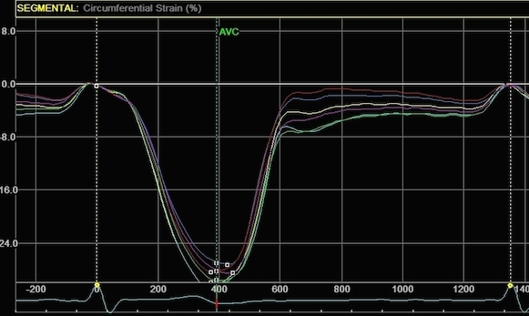
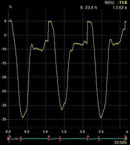
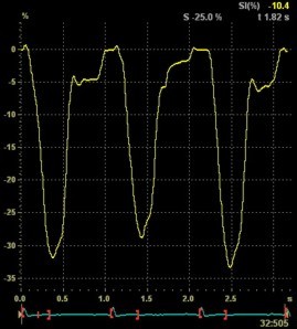
Drift. The strain curves can be seen to drift downwards from cycle to cycle. This, of course is impossible, if the deformation did not return to zero at the end of each cycle, the heart would turn inside out in the course of a few cycles. In this case the drift is caused by the integration of strain from strain rate, accumulating the errors as the strain rate values are summed from time to time.


Drift in speckle tracking

The speckle pattern will not repeat perfectly. This is due to both true out of plane motion (rotation and torsion relative to apical planes and longitudinal deformation relative to short axis planes) and to small changes in the interference pattern. But the frame to frame change is small, and the approach to recognition is statistical, the basic algorithms are shown here. Still, small inaccuracies in tracking may cause over all drift in the tracking. This is due to the fact that tracking is done from frame to frame, so the tracking in one frame starts at the position of the kernel decided in the previous frame. If there is a non random element of appearance and disappearance of these speckles, there will be an over all drift of the kernel relative to the myocardium.


Drift in ultrasound. As speckles disappear out of plane, or by changing interference pattern, this may cause less than perfect tracking. The kernel is defined in frame 1, indicated by the red rectangle. In the next frame, due to out of plane motion, or simply changes in reflectivity some of the speckles disappear or have lower intensity in the next frame due to complete or partial out of plane motion in the B-mode image.  Then the kernel may find a slightly different area as the new kernel position. (Especially if the tracking is done by the sum of absolute differences where the identification rests with the summed intensity within the kernel area). In frame 2, the true kernel motion is identified by the dark grey rectangle, the tracking, however, identifies the new position as the red rectangle. Some of the speckles above the kernel have decreased in intensity, while the speckles below have all increased. In frame 3, further changes in speckle visibility results in further  slippage, i.e. slippage in relation to frame 2, which then is a larger cumuated slippage from frame 1.  Two speckles from frame 2 above the kernel have disappeared, four speckles have decreased in intensity. Two speckles below the kernel have increased. The true position of the kernel from frame 1 is indicated by the light grey rectangle, the position of the red kernel from frame 2 by the dark grey rectangle, and the tracking by the red rectangle.

This means, however, that the with lower frame rate, the changes from frame to frame are greater, resulting in poorer tracking. Higher heart rate (f.i. in stress) will result in the same, as the number of frames per cycle will be reduced, i.e. lower relative frame rates.

Thus: speckle tracking is frame rate sensitive:
  1. Too low frame rate will result in too great changes from frame to frame, resulting in poor tracking. This may also limit the use in high heart rates, as the motion and thus frame to frame change increases relative to the frame rate.
  2. Too high frame rate is obtained by reduced lateral resolution, and thus resulting in poorer tracking at least in the transverse direction. If the lateral resolution is low,  the interpolation will result in a "smeared" picture as shown here, with speckles that are nor so easily tracked in the lateral direction. In addition the lateral resolution decreases in depth with sector probes, making lateral tracking at greater depths doubtful. The poorer the lateral resolution, the poorer tracking in the lateral direction, and the more angle dependent the method becomes.
Thus, both too high and too low frame rate may affect speckle tracking adversely. With the present equipment, the optimal frame rate seems to be between 40 - 70 if image quality is good, slightly higher with poorer image quality.

This is a fundamental property of speckle tracking,  and the drift from start of cycle to end of cycle may actually be used as a criterion for quality of speckle tracking. And even more advanced comparing tracking forwards and backwards through the whole cycle , f.i. by cross correlation. It may be less with a higher frame rate. (Although that will lead to more angle dependency). If the speckle tracking is used for calculating a velocity field as the primary variable, as in 2D strain, the integration to displacement an strain will result in further drift by cumulating small errors. In addition undersampling is a property of low frame rate, i.e. B-mode. This reduces peak velocity, and the peak values is even more reduced if smoothing is applied before integration as it is in 2D strain.

Drift in tissue Doppler


In tissue Doppler, the package acquisition of colour Doppler, results in drift from one package to the next, as shown below.

Integrational drift in package acquisition. The curve is a displacement curve. Ultrasound pulses are shot in packages of at least two pulses, and both pulses contributes to the velocity estimate, as described in the basic ultrasound section on colour Doppler. Thus the velocity is an estimate for the package with a duration of 1/PRF, and the velocity of motion is extrapolated for the interval between packages, i.e. 1/ FR. From the figure, is is evident that integration of these velocity samples will deviate from the true values in between packages: In this case there is negative drift in systole, positive in diastole, but the end result is unpredictable. The repeating pattern, however, will ensure that there may be a net positive or negative drift from heart cycle to heart cycle, which is more or less linear. The drift within  each heart cycle, however, is not linear.

This effect is not only due to the mathemathical integration of displacement from velocity, it is actually also a property of tracking by tissue Doppler, as the position of a kernel is calculated from the position and velocity in the previous frame. (this is in reality the same thing). A frame rate of 1 KHz would to some degree eliminate this. Then each velocity could be calculated by single acquisition i.e. from one frame to the next, without the gaps due to FR being much lower than PRF. This has been shown to be technically feasible (215).

Integrational drift

Any method that measures instantaneous values, and then integrates these measurements to an integrated value, is prone to drift. Random errors will cancel out, but non random errors will accumulate. Drift is thus a phenomenon of the modalities of displacement and strain where values are cumulated by integration of instantaneous curves. It results from the accumulation of small non random errors. In tissue Doppler, the package acquisition is a special mechanism for drift, as described below. But, drift occurs in speckle tracking also. Here it is related to the quality of tracking as discussed below. Out of plane motion and small shifts in probe position or heart position (respiration) may contribute, as may changing reflexivity of structures due to changes in fibre direction as described below.


Drift. The cumulation of non random errors by integration leads to the curve drifting from cycle to cycle. End cycle strain however, has to be zero.

If total strain at end diastole is different to zero, the heart would either diminish or increase in size. This is obviously nonsense. (Even with minimal changes this would lead to the heart either disappearing or growing to the size of the whole body in a matter of hours. The same is true of displacement. If the end diastolic displacement is different from zero, the heart would walk away from the patient in a short time.)

And even if total strain is zero at end systole, each region also have to end with zero strain and displacement at end diastole. Else, this would be equivalent to a shape change that would turn the heart inside out in a short time. Thus, end diastolic strain has to be zero, and this condition can be used to compensate drift.

Drift can thus be compensated in post processing, from the necessary condition that strain at end diastole (end cycle) has to be zero.

Either the value can be reset at the end of each cycle. This will not compensate for drift during the heart cycle, and may be seen by a distinct step in the strain curve at end diastole. A smoother correction is to apply a linear correction during each heart cycle, by calculating the slope  of the baseline from the "step" at the end of the cycle and subtracting this slope from the baseline values. This correction is based on the assumption that the drift is linear during each heart cycle, which is an approximation, but not completely true, as seen in the example above where drift is probably more sinusoid shaped.

Resetting at the end of each heart cycle gives more ugly curves, but does only correct what is known to be false. Linear resetting will result in correction also during the heart cycle, but this is presumptuous. This principle is illustrated below.


a: normal strain curve.  b: strain curve with drift, the curve does not end at zero at end diastole. c: Resetting, by simply forcing the curve back to zero at end diastole, will not change peak systolic strain, but will prevent the drift to carry over to the next heart cycle. However, if there is drift during the heart cycle, this drift affects peak systolic strain as well, as indicated in b and c. d: Linear correction can be applied as the slope from beginning to end systole can be calculated from the end systolic drift. . e: The slope values can then be subtracted from the strain values, thus forcing the curve back to a shape without drift. This will correct also values during the heart cycle, thus giving corrected value for end systolic strain. This correction, however, is presumptuous, and rests on the assumption that the drift is linear throughout the heart cycle, which is probably not the case in general.


Strain without drift compensation. It is evident in the image to the left that the strain curve  drifts from cycle to cycle. The drift may be both downwards and upwards, in this case downwards. Drift compensation by resetting the curve to zero at the beginning of each heart cycle. This is evident by the vertical line at end diastole. Comparing to the image left, peak systolic value at cycle 1 can be seen to have the same value, as no drift is compensated during the heart cycle.The resetting prevents the drift to affect later heart cycles, so cycle 2 and 3 have similar peak systolic strain as cycle 1, far lower and stable than without compensation.
Linear drift compensation is applied linearly during the whole period. This results in a further correction, as values during each heart cycle are adjusted as well. In cycle 1, the peak systolic strain is lower (in absolute value) than without or with linear compensation. In addition, cycle2 and 3 have lower peak systolic values than with resetting at end cycle, although this may not be the real case.


Thus, linear drift compensation affects peak systolic strain unpredictably, and not necessarily in the correct direction.

Method for drift compensation should always be reported in clinical studies.


Specific limitations in measurement

The measurement in itself will have specific limitations, related to measurement precision. There will always be a lower limit of the relative measurement precision, and the measurement variability within this precision comes out as random noise. The level of noise, (and the precision), will depend on the methods used.

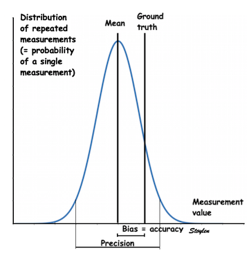
In addition, there might be a bias; even with good precision, the means of repeated measurements may differ between methods (and ground truth). If there is a ground truth (as in simulations) or a "gold standard), the difference on measurement means is the method's accuracy, and the bias is a systematic error. This is due to systematic differences between methods, but may also be due to compensation methods for random noise, as well as presence of non random noise.


Accuracy (measurement accuracy - not to be confused with diagnostic accuracy) and precision of measurements. 

As the limitations are technical, there are technical causes for both random noise and bias, so this can differ between methods. In the following, the technical issues related to measurement are discussed.


Sampling rate


The basic problem of sampling rate is related to measurement of peak values. If the sampling rate is much lower than the rate of change of peak values, the probability of hitting the peak is low, and on average, the measurement will underestimate peak values, called undersampling. Undersampling will also increase variability, by introducing a random element in hitting the true peak value (74). On the other hand, if the rate of change is slowest at peak, the sampling rate does not matter much. The principle is shown below.

The effect of sampling rate. The true curve is shown left, with the sampling points shown on the curves as well as below the curves. To the right are the sampled (reconstructed) curves, from interpolation between the values at the sampling points.  Top: low, and bottom: high sampling rate. It is evident that the sampling rate at the top fails to hit the true peak value, and the peak value shown is underestimated. In addition, hitting the true peak is a more random process, so undersampling will also increase variability. Bottom, the sampling rate is doubled, interpolating sampling points between those at the top (you may measure with a ruler, if you want) and hitting the peak fairly well. The reconstructed curve resembles the original much more closely.


In post processing tissue velocity data, the sampling frequency is equal to the frame rate. The shorter the duration of the event to be measured, the higher the frame rate ought to be.

Thus, short duration events need a high sampling rate, not only for measurement of peak values, but also for reproducibility of these peak values (74). Analysis by decimating tissue Doppler images, showed that peak systolic velocities had both reduced mean values as well as reduced reproducibility, at frame rates below 70, isovolumic indices below 100 (74). However, this is not the only problem. Temporal filtering used to decrease random noise, also reduces the effective frame rate, so even if the frame rate is sufficient applying temporal filtering will then reduce peak values and increase variability (77). Tissue Doppler has a frame rate of ca 100, B-mode 50 - 100 in a full sector image.

Thus ideally, increased temporal filtering should be compensated by increased frame rate.

Frame rate can be increased to about 150and 90, respectively, but at the cost of lateral resolution which affects both tissue Doppler, inducing artifacts, as well as  speckle tracking in the ability to track laterally as shown also for 2D strain, which also increases angle dependency of speckle tracking.

However, it is important to realise that this is relevant for the measure of peak values. To detect the events and measure duration on colour images, the frame rate only needs to be adequate to detect changes from positive to negative values consistently 50 FPS is generally sufficient.  The temporal resolution of time measurements, however, will depend on the frame rate rate, 50 FPS gives a resolution of 20 ms.

It important that strain is less frame rate sensitive, as the rate of change is lowest at end systole, comparable to ejection fraction. In fact, ejection fraction can be fairly reliably measured with a sampling rate as low as 1/3 sec by MUGA. Strain has a similar time curve. This means that reduced sampling frequency is less important. However, one study did find that frame rate had an impact on measured strains (124) in tissue Doppler.

Frame rate should always be reported in clinical studies.

Frame rate in WMS

In visual assessment, the main limitation lies in the eye, which usually has a temporal resolution of 80 - 100 ms (24). However, with modern equipment this limitation can be overcome, by slow replay, which makes the temporal resolution of the eye equal to the B-mode frame rate. This still means that the limitation is the B-mode frame rate.

In order to achieve optimal temporal resolution, it is customary to stop the loop and scroll through it frame by frame. This usually shows segmental dyssynergy as failure to thicken during the first frames of each systole. But this again means that wall motion scoring is more dependent on early failure to thicken/shorten, i.e. the timing of onset of contraction, than on peak thickening/shortening (strain) or peak thickening/shortening rate (strain rate). This  in fact doesn't measure exactly the same thing, but again is often dependent on the method of the individual user.


Random noise

As strain rate is the difference between velocities, while the noise is the sum of the relative errors of the velosity measurements, the signal-to-noise ratio is far less favourable sin strain rate imaging than in velocity imaging.


Velocity measures with some amount of noise.
Unsmoothed strain rate curves from the same loop. The increase in noise is evident.

Random noise will tend to increase peak values, if measurements are done at the top of the noise spikes, while it can be corrected visually if placing the points of measurements in the average line. In the original post processing application  no smoothing was applied. That meant that the original studies were done by visually correcting for noise.

The experience from the HUNT study (153), seem to show that strain rate by tissue Doppler is a more noisy method for strain rate than the others, including segmental strain, giving higher peak strain rate (probably due to noise peaks) and wider standard deviations (variability) as shown in the comparison study. Strain did not differ, showing that the integration to strain is efficient in eliminating random noise.


 However, it's an illusion that there is less noise in speckle tracking than in tissue Doppler. This illusion is created by the extensive smoothing used in speckle tracking applications.

As explained above, the speckle tracking starts with generating a velocity field, by measureing the speckle displacement and dividing by the inverse of the frame rate (the sampling interval). This velocity field is then used for calculating the strain rate (by spatial derivation) and strain (by temporal integration) as described above.


We did an initial evaluation of an earlier version of this application in February 2004, comparing the longitudinal motion and deformation measurements by this application with those obtained by tissue Doppler, in separate images. The study consisted o0f 20 patients with a wide range of function.


Strain rate and strain, comparison of 2D strain and Tissue Doppler. There is a considerable spread between methods, but most probable due to variability of especially of tissue Doppler. There 2D strain gives lower values than DTI, and this tendency increases with increasing strain rate/strain. The term "CEB" meaning "computerized eye balling" was an early term to describe the application.

When measurements was sorted in quartiles, Concordance was only between 27 and 34%. Feasibility was the same with 2D strain and TVI. Further investigation was not undertaken at that time, as the application was modified in later versions. Other authors have found a much better correspondence between TDI and 2D strain (73), with correlations of 0.94 and 0.96 for strain rate and strain, respectively. However, as seen by the curves in the figure below, both data sets are analysed by the 2Dstrain software, and thus subject to the same high degree of smoothing, so the results do not reflect independent analysis.


From a validation study where tissue Doppler and 2D strain derived strain rate (left) and strain (right) values were compared. However, as can be seen
from these curves, both curves are very smoothed and concordant. Thus, much of the concordance must be assumed to be due to smoothing, as both
methods were processed by the 2D strain software, and not by independent analysis software. Adapted from Modesto 2006 (73).


This is illustrated below:

The lines looking smoother, is a function of the averaging function used in the algorithm, the application will do the same to tissue Doppler data.


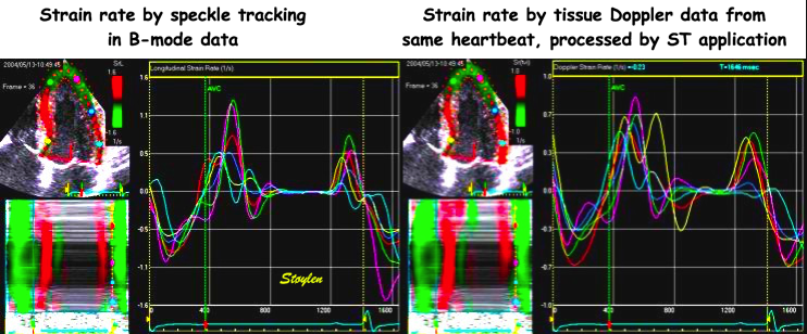
Strain rate curves from speckle tracking and tissue Doppler from the same cine - loop.  The same smoothing is applied to both, showing that smoothing of the curves is not the result of the robustness of the algorithm, but of specific temporal and spatial smoothing applied by the application. The curves differ somewhat (but not too much), as strain rate is calculated with different angle and lateral resolution.

Another study by Cho et al (148) finds only correlations of longitudinal strain by 2DS and TVI with MR tagging of 0.51 and 0.40, respectively. This may reflect the real precision of both methods (and of MR tagging as well?) but then the correlation between the methods cannot be higher.

How to deal with noise?

Linear regression of velocities:


Instead of measuring just the velocities at the ends of the offset distance, strain rate can be calculated as the slope of the regression line of all velocities along the offset distance as described in detail in the basic concepts section.


True strain rate: blue, strain rate by velocity difference: green, strain rate by linear regression: red.


Increased strain rate length (offset distance).

Increasing strain length,  will increase the difference between v1 and v2, while the error of velocity measurement will remain the same, thus improving the signal-to-noise ratio. With the integration method, an increased strain length will result in a larger number of point velocities that are averages, thus increasing the effect of integration. Still, each strain measure results in a value that is assigned to the mid point of the strain length.

Spatial smoothing (increased ROI size)

In the ROI each pixel represent the mid point in a strain length. Increasing the ROI size, will result in more pixel values being averaged, thus reducing random noise by averaging.However, increasing ROI size induces a risk of including areas of non random noise (clutter).


Same ROI, but increased strain length. The effect of strain length can clearly be seen. Usual default offset at present is 12 mm. ROI size. With strain length 4 mm, the effect of averaging more samples is evident.  Usual default is 12 x 6 mm at SL 12 mm.


Illustration of how both strain length and ROI size reduces spatial resolution. each strain length is represented by a point in the middle of the length. In principle the radial (depth) resolution should be ROI length + Strain length, but as shown the effect of the points outside the ROI decreases with the distance from the ROI with the regression method.


The increased noise due to shorter strain length is evident also in these parametric images.

Ideally, the strain length plus ROI should be as great as possible, giving the highest possible velocity difference to ensure the best signal-to-noise ratio. As there may be little added information by entering into sub segmental resolution, the resolution may be as low as the length of one segment. This will give the segmental strain rate and strain, although measured along one ultrasound beam. However, this also increases the risk of including areas of reverberations or drop outs, and thus, reducing random noise at the cost of increasing non random noise.  This is indeed true of all methods for spatial averaging.

Temporal smoothing

Temporal smoothing is achieved by averaging measures from more than one frame. this can be done by a simple averaging, or by a weighted averaging where the samples may be weighted bu a gaussian distribution of weights. In addition it is customary to use the sliding window technique, which can average more frames without reducing the effective frame rate quite proportionally.

Simple averaging vs Gaussian averaging. In simple averaging, each point is taken as the simple average of the three points in the sample, where each point is weighted equally. In this example of Gaussian averaging, each point is the average of three samples as well, but in calculating the average, the samples are weighted by the distance from the centre point according to a Gaussian curve. This maintains a better temporal resolution. 

Illustration of the sliding window technique for temporal smoothing. The original curve (black) is noisy. Averaging the three first samples (1 - 3; green), results in an average curve. Instead of moving to the next three samples, the smoothing window then moves to frame 2 - 4, taking a new average (red), then to frame 3 - 5 (blue), frame 4 - 6 (brown) and finally to 5 - 6 (cyan). the averages of each window are shown as the dots of the same colour, and the resulting smoothed curve is shown in grey. The more samples in each window, the smoother the curve, but the lower the effective frame rate, although the effective frame rate is not reduced as much as the number of frames in each window.


Effect of temporal smoothing and strain length


A detailed treatment of temporal filtering can be found in (75, 77).

Later temporal smoothing, and in the latest software, the Gaussian temporal smoothing is implemented. Default at present is Gaussian 40 mm at SL 12 mm and ROI 12 x 6 mm. With good recordings, the curves with tissue Doppler may at present look more like this:


Left: velocity recordings, right strain rate with standard strain length and ROI settings and Gaussian smoothing over 50 ms.

It is a far cry from the raw data presented at the beginning of this discussion, but it should be kept in mind, that the underlying raw data quality is more like that.


Integrating to strain


Another method for temporal smoothing is using the integrated strain instead of strain rate. As noise is random, the summation of strain rates from each frame will statistically even out the noise spikes and throughs:


Effect of temporal integration. Left unsmoothed strain rate, right strain from the same dataset. As the noise is random, the summation will eliminate the random variations, resulting in smooth curves.

  The main problem with any form of temporal smoothing is that it reduces effective frame rate, and may lead to undersampling.


Averaging more than one heart cycle (Cine compound):

Which in general is a bad idea.
Random noise will not repeat from heart cycle to heart cycle, and thus averaging more than one consecutive heart cycle, will eliminate random noise. As can be seen from the recent comparison of methods in the HUNT study (153), peak systolic strain rate by tissue Doppler is much more sensitive to noise than other methods. This can be seen from the fact that the average (absolute) peak values are much higher then other methods, while the standard deviations are correspondingly wider. Thus the peak values incorporate noise. Systolic strain, on the other hand, are quite similar, showing that the increased peak values disappears as noise is integrated sto strain as discussed above and that the higher peak values are incorporating noise peaks.

On the other hand, averaging heart cycles has several disadvantages:
  1. The frames will not be at exactly the same time point in the cycle, and thus corresponding franes will be from slightly different points in the cycle, and thus averaged. This effect is in fact similar to temporal averaging, and results in a similar reduction  in effective frame reate, and may lead to undersampling.
  2. As there is significant beat to beat variation in cycle length, later events in the heart cycle will occur at different intervals from the R-wave. Systole and diastole varies differently with respect to RR-interval, especially at HR < 100 (29), it will especially affect the time around end systole / early diastole.This may lead to bizarre results as seen below.
  3. Cine compounding by automated methods will always sample three consecutive cycles, and if one beat is of low qualituy due to motion or respiratory artefacts, or even as an extrasystole, the compound curves will include the artefact.


Native recording, showing four cycles. (Healthy child, HR around 90). It is evident that there is variation in heart rate, as it can be seen by the increasing fusion of E and A waves.
Cine compound x 2, i.e. each cycle shown in a compound of two cycles.  Systolic peak velocities does not change much, but e' wave velocities are almost halved, due to the averaging of E waves that are at different relative positions in the cycle.
Cine compound x 3, i.e. each cycle shown in a compound of three cycles.  There is not much change from cine-compound x 2, and still e' waves are very different from the native loops.


Velocity curves from the septum.  There is substantial noise as well as fusion of E and A due to beat 2 being an extrasystole at the end of cycle 2 (arrow).
Resulting in a high noise spike in the strain rate signal,
which again leads to a substantial artefact in the strain curve.


When this artefact is shown in a non-compounded image, it is limited to one cycle, and it it fairly evident that this cycle should be discarded.
Cine compound x 2, extends the effect to two cycles
and cine-compound 3 extends the effect to three cycles, and in this image, it is not evident which cycles are representative.

Basically, if one is concerned about peak values, averaging peak values from three cycles will be more robust that automatically creating a cine compound cycle, and especially if cycles that deviate are eliminated. Thus, one is not restricted to three consecutive cycles. Cine compound may seem an attractive way of averaging three cycles, and then being able to reduce the number of measurements to one set in a cycle that is the average of three, but then the following caution should be observed:

  1. It should only be applied to systole. Also, velocity measurements are fairly smooth already, while strain rate is noisy and is the case where one profits most. Thus peak systolic strain rate maight be the one case where it it feasible and favorable. Strain curves are fairly smooth already, and cine compound will not add anything.
  2. It should only be applied where there are three consecutive cycles of good quality, but as can be seen above, the noise is not very evident in the velocity curves, and if cine compound is applied before conversion to strain /strain rate, the artefacts may be less evident.

Smoothing in 2D strain

As said above, there is just as much noise in speckle tracking as in tissue Doppler in the raw data. There is applied both temporal and spatial smoothing to overcome this, and the approach is different from the methods of tissue Doppler described above.

The main method is a spline or polynomial smoothing along the whole region of interest (ROI).

Spline smoothing. The whole wall with all six segments are the ROI, and the spline smooting is distributing the values over the whole ROI. The segments still remains different, due to the spline distribution


This is equivalent to the linear regression along the strain length, but using polynomial regression, and extending the strain length to the whole ROI. This means that all segments are interdependent, not independent as in tissue Doppler (and only neighboring dependent as in the segmental strain method). It will also result in temporal smoothing, as temporal differences, both random (due to random noise) and real (due to temporal inhomogeneities - both normal and pathological) may be smoothed away.

The AV plane is the heaviest feature that is tracked, and contributes the most to the motion, which is then distributed along the whole ROI by a curve fitting along the mid ROI curve, resulting in a smoother transition from segment to segment, distributing the deformation along the ROI. Thus, the 2D strain application does not reflect pure speckle tracking, but also a great amount of model fitting. The spline smoothing is weighted, being least in the basal segments, most in the apex, which may be a way to compensate for some of the curvature effects in the apex, but that means tat adjustments in the base will affect measured strains in the apex.


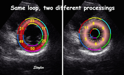
The spatial smoothing, however, is adjustable. By default, the smoothing is medium, and can be adjusted to both maximum and minimum. However, in earlier versions of the software, the regulation of the smoothing did not carry over to the measured segmental values displayed in the quad screen view. Thus, segmental values remained medium smoothed, and values with less smoothing had to be taken from the traces. This problem seems to have been fixed in a later version of the software (2011), but this means the software version should be taken into account. Also, the adjustment seems to be small, compared to the total amount of smoothing.


This is illustrated below.

False speckle tracking. This is due to spatial smoothing in the algorithm, in order to reduce the imapact of drift and other sources of noise. The smoothing, using longitudinal information from the AV-plane motion, distributing it along the ROI by a spline function, creating a kind of "model" of the motion.  As can be seen, in this image it "tracks" even if there are no speckles. This, however, is not true tracking, the bullets move according to the model calculating where they should be. Thus, there is  only "false tracking", and the true local tracking cannot be fully assessed visually, and the visual quality assessment of tracking can be deceived.


The smoothing may be adjusted in the application, but even minimum smoothing will result in measuring high strain values in empty space.


Segmental values from this tracking. Left: medium (default) spatial smoothing, right: Minimum.  This was done in the latest software version (2011), where values and traces carry over to segmental values after adjustment of smoothing, but the effect is small, compared to the total amount of smoothing.


This example was obtained by manual override of the automated positioning of the ROI, as well as manual override of the automated quality check, which suggested rejection of all segments. However, the application did track, as can be seen above, left, and these images are to show the general principle.


Inferior infarct in two chamber view, being akinetic in the basal inferior wall, although with considerable passive motion due to tethering


2D strain (left) vs. tissue Doppler (right) in an inferior infarct, analysed from the same cine loop recording.  The akinesia in the base is missed due to smoothing. In this case, as there is dropout of the whole anterior wall, the smoothing may be harder in the remaining three segments.  Also, in basal infarcts, the effect on AV-plane motion is less (40) as shown above.

Fundamental limitations of speckle tracing

The speckle tracking method has fundamental limitations, just as tissue Doppler

It must be emphasized, however, that new computational techniques has served to increase  both focus, line density and frame rate of B-mode, especially after leaving the crude MLA approach, thus improvements in 2D speckle tracking may be expected as well. (And previous study results be rendered less valuable). This means that some of the reservations towards speckle tracking in terms of frame rate and lateral resolution is less important. This, however, do not lead more validity to earlier results.

Quality evaluation of speckle tracking


Basically, the quality of the speckle tracking can be assessed visually, by evaluating how well the kernels follow the tissue motion. This is facilitated by slowing the replay, or stopping and stepping the frames (a method that is strongly recommended in stress echo evaluation as well). In the basic application, this is feasible, as each kernel tracks independently. (This is not always the case in more advanced commercial applications, as will be discussed later.) Independent tracking also gives the possibility to replace a kernel that is not optimally placed:


The kernel is in a reverberation in the lateral wall, and will not track, thus both the segment below and above the reverberation will show artefacts.
Adjusting the position of the kernel manually, allows speckle tracking despite the reverberation, if the kernel remains outside the reverberation during the whole heart cycle.

Thus the position of the kernels can be adjusted. If this is not feasible however, the segments can be discarded from analysis. Additional software may give automated quality control. The method used in the HUNT study checks quality by tracking forwards and backwards, comparing the tracing both ways by cross correlation (151), or by the difference between backward tracking and start of forward tracking (127, 128, 151). It still remains unsolved which method (including visual assessment) is best.


The fundamental limitations of speckle tracking, however, apply.


The limitations of the combined method is the same as for echo in general issues related to image quality, and the general limitations of segmental strain.


It has been considered a problem that the combined method is not commercially available, at present it is a research tool at the Norwegian University of Science and technology. It has been criticized by some, that the results are not useful, as they are not transferable. I consider this criticism only partially valid.
  1. Firstly, this is a research tool so far for doing research into and comparing speckle tracking and tissue Doppler. And the speckle tracking is "pure" speckle tracking, not advanced applications utilising a lot of computing to achieve results. The application makes it possible to compare tissue Doppler, speckle tracking and the combination directly (151), and as shown below.
  2. The HUNT substudy showed little bias between methods.
So far, the two data sets could be combined in different ways, not limited to the application described above. Further research should be undertaken to assess this.

It seems rather absurd in the long run, that having access to high quality grey scale tissue data as well as high frame rate tissue Doppler data in the same loop, the quality of measurements will improve by discarding one of the data sets.

The first step in processing will be the quality control of the tracking, as described above. The application has built in automated assessment of the quality of tracking, with methods similar to the ones above. Thus the application will suggest acceptance or rejection of the segments in the view. However, the segmental quality assessment is compared to the average, there are no absolute criteria, so tracking should still be evaluated visually, and segments that do not rack, should be excluded manually.


Loop from another patient. Tracking seems fair, visually.
Automated quality assessment accepting the tracking results from all segments. The assessment is presented as a suggestion, and manual acceptance is required, i.e. the accept button has to be pushed in order to process.
Here is poor tracking in the apical lateral segment due to near field reverberations, and on the other hand, exaggerated tracking due to side lobes. In this case, the application suggested to accept all segments, which would result in the values as shown.  And the poor tracking does not reflect in the values, due to the spatial spline smoothing in the application.


However, the apparent tracking may be due to the spline function, and will not necessarily reflect the true tracking in a local area. 


Specific limitations in strain and strain rate imaging

Measuring deformation in one direction at a time in a 3dimensional object results in specific problems as well.

The angle problem in strain.


When the direction of the motion is at an angle form the ultrasound beam, or the tracking direction, this will result in angle distortion, as shown in the basic ultrasound section and the Doppler section.

The tracking, however is affected differently:
In distance and motion measurement, the measurement increases with the angle:


which means that also the velocity calculated from this tracking, will increase with the angle, opposite to the Doppler effect:
In Doppler velocity measurement, the measurement decreases with the angle:


which also means that the distance calculated from this angle decreases with the angle as opposed to the effect on tracking.

Simple linear strain measurement is not affected, as both diastolic and systolic lengths are affected by the same amount, while the ratio between them remains the same. However, this argument is only valid in one dimensional strain. In three dimensional objects, there are simultaneous strain in more than one direction, and in incompressible objects, some strains will be positive, other negative as volume is constant, and thus will detract from each other as more than one strain component is measured at an angle.

The geometric angle problem

The main point of strain measurement is that strain is basically measured along one line. If this is not parallel to the direction of one of the normal strains, the alignment error may add to or detract from the main strain measurement as shown below: In an incompressible object, there is simultaneous strain in the transverse direction, in order to keep the volume constant, and the two strain components are opposite and will detract from each other (1, 2, 7). This results in further reduction in the measured strain and strain rate (7). This results in further reduction in the measured strain and strain rate (7). It is evident that the insonation angle becomes important again, as the relative contributions of each strain component depends on the insonation angle.


An object undergoing longitudinal shortening (negative strain). If the object is incompressible, there will be simultaneous transverse expansion (positive strain) as well. This means that the direction of measurement (along an ultrasound beam or an ROI) matters, the more skewed the beam, the more transverse strain is incorporated into the measurement, detracting from the absolute value of the longitudinal strain. The in between line will measure both to the same degree, i.e. zero strain, while the beams in the more transverse direction will measure increasing positive strain.

This is discussed in detail in the basic concepts section.

This is illustrated below.


Apical long axis view from a healthy person. The base of the inferolateral wall is positioned at an angle to the insonation. An M-mode line along the ultrasound beam shows positive strain, by the divergence of the M-mode lines (speckles). The wall thickening is predominant. Interpreted as longitudinal strain, this vould mean systolic elongation . dyskinesia.
Adjusting the direction of the M-mode, in this image the longitudinal and transverse strain balance, as seen by the parallel lines (speckles). This results in near zero strain. Interpreted as longitudinal strain, this would mean akinesia.
Further adjustment of the M-mode line, will result in best alignment of the line with the wall, and here there is negative strain seen by the convergence of the lines (speckles). This shows true longitudinal shortening, although if there is a residual component of transverse strain is uncertain.
In the example above, the ability of the application to track longitudinal shortening, depends on the ability to track in the lateral direction, as the wall has an angle with the ultrasound beam. However, in this case, there is poor lateral resolution in the inferolateral segment as well (reduced virtual aperture).

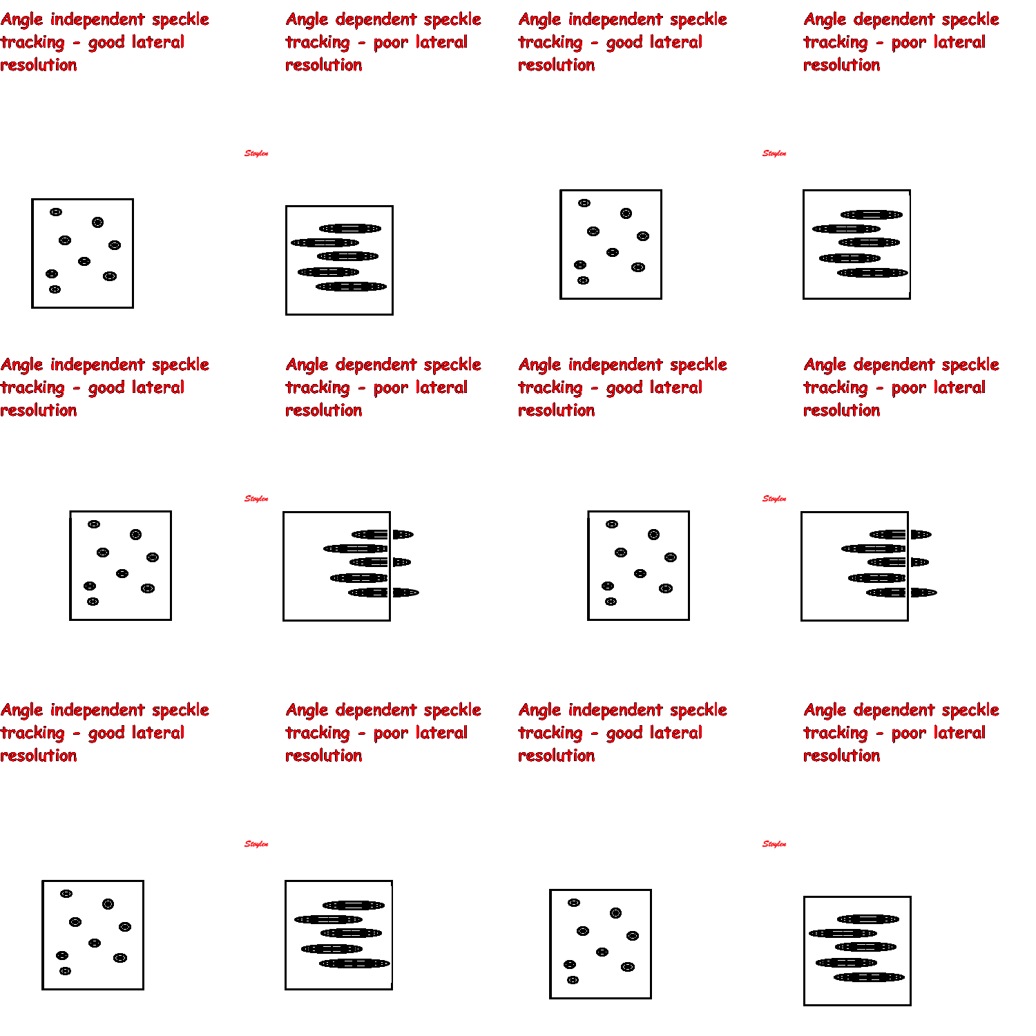
The angle independence of speckle tracling depends on the lateral resolution:

Angle dependency of speckle tracking is related to lateral resolution. Left good resolution, as the speckles move, the kernel (rectangle) follows the speckle pattern. Right, poor resolution. As the speckles move, the kernel will follow the vertical motion, due to better radial resolution. The kernel will be unable to follow the lateral motion, at least until all the kernels have crossed the kernel boundary. This mean that there is only tracking along the ultrasound beam.

Angle in speckle tracking


In speckle tracking, in principle, if tracking is perfect, there should be no angle effect, as the tracking occurs in the direction of the longitudinal shortening. However, as explained elsewhere, the lateral resolution is far poorer than the axial, and thus there is an angle dependency as well. And in practice, the effect on speckle tracking depends on many factors, such as the orientation of the ROI, the ability of the algorithm to take ROI direction into account when tracking (and interpretation) , and the lateral resolution in the image. This is illustrated below, where 2D strain is applied to the same loop as above.


Same loop as above. Apical long axis view from a healthy person. The base of the inferolateral wall is positioned at an angle to the insonation. Same loop processed for speckle tracking. Evaluating the bullets seems to show a fair tracking. The basal inferolateral segment (yellow) seems to follow fairly well, but still there is some thickening that interferes with the analysis of the shortening.
The automatic algorithm also approves all segments. Same view in tissue Doppler acquired immediately afterwards


Tracking is good by velocity curves, giving reasonably shaped curves and decreasing towards apex in both walls, with highest velocities in the basal inferolateral segment (yellow)
And they correspond fairly to the tissue Doppler curves.


Displacement curves integrated from velocity curves also show a normal pattern, also in the basal inferolateral segment (yellow) And again with fair correspondece to tissue Doppler curves


But the strain in the inferolateral segment is inverted, due to the angulation effect described above, the application measures more transmural thickening than longitudinal shortening, just as in the M-modes above
Surprisingly, in this case there is not angle distortion in the tissue Doppler strain. This is due to differences in the ROI size, placement and strain length, as well as the fact that in this method, strain is measurted along a line, not a segment.

This result is not due to the angle distortion alone, but the ability of the application to track in the direction of the wall, caused by the particularly low lateral resolution in this segment (partial near shadow effect), as seen by the width of the speckles. It is not, as some migth believe, due to inclusion of the pericardium in the RIO:
  1. Inclusion of the pericardium would include some zero strain, which would freduce the absolute strain value, but not mimic dyskinesia
  2. As seen by this tracking, the sector follows the inside of the pericardium


Angle in tissue Doppler


The tissue Doppler derived strain is more complexly affected. As velocities are reduced by the cosine of the angle, and length is increased by the same, the effect on the velocity gradient would be expected to be affected by the square of the cosine of the angle, as discussed in the basic concepts.


But it is not always the tissue Doppler method that has the greates angle problem, as seen above:


Tissue Doppler is still angle dependent, but segmental strain by tissue Doppler has only the basic limitation common to all Doppler measurement. And using it in combination with transverse speckle tracking, eliminates this angle dependency also, to the same degree as in speckle tracking (meaning that speckle tracking is not altogether angle independent).

However, drop outs and reverberations will affect the tracking, and in the lateral direction, low lateral resolution will "smear" the speckles in the lateral direction, making tracing less perfect, as can be seen in the parasternal long axis image above. It also means that the lateral tracking will be poorer with increasing depth (as the lines diverge as well as becoming wider), as also discussed in the measurements section.


In another example, the effects are opposite:


As the ultrasound beams crosses the basal septum, it is in reality mainly measuring transverse thickening, not longitudinal shortening. This is very evident from this reconstructed M-mode from the same loop. In the M-mode the motionof the specles can be seen as continuous lines. As the lines diverge in systole, speckle tracking will measure positive strain, and, if the algorithm sees this as longitudinal strain, this will be displayed as elongation - i.e. dyskinesia.


Analysis software, with a defined ROI, may to a certain degree compensate for this, as the direction of the wall is entered by the ROI definition.

The basal septum thus is more or less transverse to the ultrasound beams, and strain may be seen as positive along the beams.
As seen here, the basal septal segment, (red curve) shows apparent dyskinesia, as the basal septal segment measures across the wall, despite an attempt to define the true S-shape of the wall

reduced lateral resolution in B-mode in order to achieve a high frame rate (or indeed, 3D images), may increase angle dependency in speckle tracking by reducing the ability to track in the lateral direction. This will make the speckle tracking method even more angle dependent, although the tissue Doppler method is more angle sensitive, as the single velocity measurement is reduced by the cosine of the insonation angle, before taking geometrical distortion into account.

Thus, the angle distortion of speckle tracking derived strain, cannot be quantitated, it depends on how ROI is placed, and the ability to follow the longitudinal motion of the wall instead of the cross sectional.

 
This is the same example as shown above.
In tissue Doppler, measuring strain rate along the ultrasound beam, there is positive strain and strain rate (wall thickening) in systole in the basal septum and negative strain (thinning) in early diastole (yellow curve), as opposed to the normal shortening shown in the more apical  part (cyan). This gives an illusion of a dyskinetic segment.The problem can thus be seen to be more pronounced than in the speckle tracking application.


Thus, as we see, crosswise beams will result in inversion of strains, showing apparent dyskiesia. However, the problem is less than maintained by many. It is mainly in the apex, the base and as in this case where there is a sigmoid septum:

Strain rate 3D mapping: Angle artefact in the anterior septum due to sigmoid septum, showing systolic  positive  strain (blue - apparent lengthening) due to the angle being crosswise to the wall, in reality measuring thickening. Another patient with no sigmoid septum shows no artifact in the base of the septum. In addition, as the ventricle is not dilated, the apical area with apparent lengthening (blue) is fairly small. There is also a small area in the base where the wall curves inward.
Strain rate curves from the apex of the same patient showing it to be perfectly feasible to measure strain in the basal part of the apical segment (red ROI and curve), the area with inverted values (being in reality thickening) is fairly small (yellow ROI and curve).

It's important to realise that this double angle problem is limited to the velocity gradient method.

However, despite the well known sensitivity of Doppler to angle deviation, it is not always the case that the angle problem is greatest in tissue Doppler. In some cases, the angle problem may even be worse with speckle tracking than with tissue Doppler, due to the complex functioning of the speckle tracking algorithm:


Amount and method for temporal averaging should always be reported in clinical studies.

Insonation angle deviation in different parts of the ventricle_
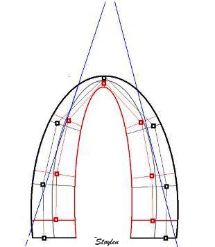
Which segment that is most in alignment with the ultrasound beam, may vary  with LV depth as illustrated here. 
LV shape also is important in determining the degree of wall alignment.

It has been maintained that strain and strain rate cannot be measured in the apical segments, but from the illustrations shown above, this is not necessarily true for all patients on a segmental level, and the apical segments may in fact be the ones showing best alignment in some cases.


However, the apex seems most susceptible in the HUNT study, but the problem was solved by the ROI tracking the myocardial motion.


In post processing, the main point is to exclude segments with to great angle deviation from analysis, at least other than timing by parametric
In some instances the angle problem is due to imperfect alignment (foreshortening), if the probe is not positioned properly over the apex. (As indeed may be necessary to obtain an acceptable window). In that case, the angle problem can vary along the wall as shown below:


Less than perfect alignment with the apex, results in a, angle along the inferior wall in this 2-chamber view. It can be seen that the wall apparently is curved, and that the alignment is better in the basal than the apical half.

This has different effect in the different parts. Basally, there is a normal strain rate curve (yellow). Apically, the systolic strain rate is reduced to half, due to angle distortion (red). In the midwall, there is a normal peak value, but the systolic curve is cut off, resulting in zero values in the late systole (cyan). as the bent area moves into the ROI.

This is also apparent in the curved M-mode, showing an area of apparent a- to dyskinesia in late systole in the midwall.

Using timing information, especially the shifts between positive and negative strain rate, on the other hand has been proposed to overcome the angle limitation. This, however, may be problematic if the alignment is less than perfect, in a way tat the angle between the ultrasound beam and the wall varies through the heart cycle, as shown in the midwall segment in the middle image above.


Variable insonation angle during the heart cycle

In individual cases, there may also be angle problems in other levels, especially the inferior wall in the care of foreshortening. The angle deviation may apparently vary during the heart cycle.


Two chamber view. The apex is in fact outside the sector to the left, and the inferior wall appears to have a break in the midwall. The middle part is transverse to the ultrasound beam, and here the measured strain rate will be wall thickening (positive strain rate), as shown in the diagram, longitudinal shortening (negative strain rate; orange arrows) in the apex and base, transverste thickening in the midwall (positive strain rate; cyan arrow). In the curved M-mode, the area of positive strain (transverse thickening is seen to move with the wall. The pattern may resemble a reverberation, but doesn't last throughout the heart cycle, and the time course is not horizontal.

The motion of the distortion area suggests how to deal with this artefact by making the ROI track the myocardial motion, as shown here.

Tracking the ROI:

Commercial software have the option of tracking the ROI manually, but the tracking could be done by automatic methods as in the NTNU application. The tracking eliminated the systematic angle problem in the apex in the HUNT study.
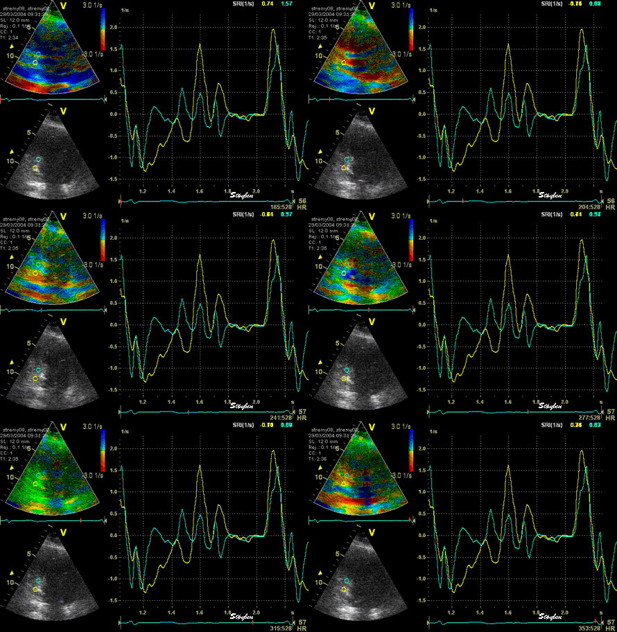


The same loop as above, showing normal strain rate curve in the base (yellow), but abbreviated systolic strain rate curve in the midwall, as the area of transverse strain moves into the  ROI.

The same ROI placement in start systole as left, but now the ROIs are made to track the myocardial motion  through the systole. Thus, the midwall curve improves, showing normal strain rate through systole, demonstrating the the finding in a is an artefact. It also demonstrates that tracking makes little difference in a normal strain rate curve (yellow), except maybe in the apex.

Thus, as opposed to stationary artefacts, tracking may help to keep the ROI outside the path of moving artefacts, but of course if the ROI is trackiong into a reverberation, the results will be worse
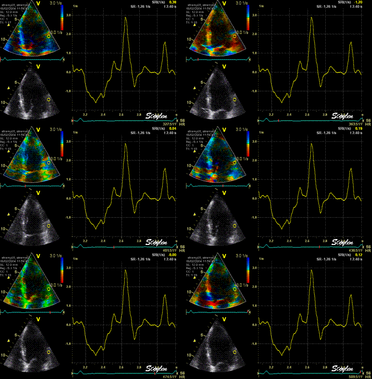


Normal strain curve below the reverberation. The ROI is stationary in space.

Same ROI as left, but the ROI made to track the myocardial motion, passing through the reverberation during systole, and strain rate curve can be seen to be cut out and inverted in that period.

Thus the value of tracking the region of interest depends on the quality of the data. 

Curvature dependency of 2D strain

The longitudinal values that are obtained by the 2D strain application are curvature dependent, as shown below:


Curvature dependency of strain measurement. If the ROI is curved, the midwall line will move inwards, and thus shorten, even if there is no shortening of the segment. This will result in an apparent shortening of the segment itself, adding to the real longitudinal shortening. This curvature effect is dependent on the curvature, the width and the widening of the ROI.

Curvature dependency of strain in 2D strain by speckle tracking. The two images are processed from the same loop, to the right, care was taken to straighten out the ROI before processing, while the left was using the default ROI. In both analyses the application accepted all segments. It can be seen that the apical strain values are far higher in the right than in the left image (27 and 21% vs 19 and 17%).  However, the curvature of the ROI even affects the global strain, as also discussed above in the basic section.

The width and thickness as well as curvature of the ROI is non standard, defined ad hoc. In addition, the ROI width is uniform from base to apex, while the myocardium is thinner in the apex, giving a discrepancy between ROI width and wall thickness. As the curvature effect is also a function of ROI width, this may add to the curvature effect. This effect may account for the observed base-to-apex gradient of strain values observed in some studies. The combined method (and indeed tracking of segment length by speckle tracing alone without TDI by the same application) is curvature independent as shown below.  It may be the reason why some authors find a base-to-apex gradient in the strain values obtained by this application, while we did not in the HUNT study.
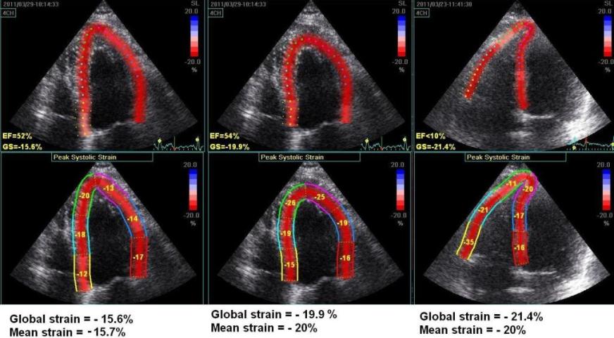

Another instance of the curvature dependency of measured values. The left image is processed with fairly straight ROI in the apex. The middle image is the same loop processed with more curved ROI, in both cases the application suggested acceptance of the tracking in all segments.  AS opposed to the above example, in this case the global strain is severely affected by the ROI shape as well (.15.7% vs - 20%). To the right is shown another loop from the same patient, centered on the right ventricle. In this case, the values of the septum is quite similar to the values in the left image, but differs from the middle image. The interesting thing is that the global strain itself is different from the mean strain calculated from the segmental values.

This may affect the regional strain as well, as the curvature dependency may assign higher values to akinetic segments as shown below:


Small apical infarct. Admitted with a history of pain, but free of pain and with normal ECG, but elevated Troponin (analysis results not ready till he had new pain) at the time of admittance.  This Echo at admittance was initially considered normal, even though by retrospective evaluation there is a small area of hypokinesia with delayed onset in the apex.  He then had recurrent pain after a few hours, with ST-elevation.
The colour M-mode clearly shows the delayed onset (Apical part starting blue), and the time delay can be measured. Also. the colour is lighter, and more seckled, showing qualitatively thet the contraction is reduced.


Tissue Doppler based strain rate and strain showing hypokinesia in the apex (yellow and red curves) , peak systolic strain of - 5% and -8%, strain rate of - 0.35 and -0.8 s-1 both segments with post systolic shortening, as contrasted with normal deformation in the base (green and cyan). This is an indication of a small ischemic insult at the time of the first pain episode as also shown by the troponin results.


Angiography at the time of recurrent pain showed a tight LAD stenosis (top), confirming the strain findings, it was treated with PCI and stent (bottom) in the same procedure. Strain and strain rate values were normal after one week.


2D strain of the same recording (B-mode loops without TDI). The curved M-mode gives apical strain of  -14 and  -15%, i.e. borderline normal. This was the default ROI.
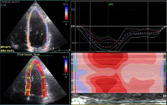

Adjusting the ROI making the apical segments straighter, reduces apical strain to -9 and -11% (borderline abnormal)
Both images were made with default (medium) spatial smoothing, but the values did not change more than 1% by reducing smoothing to minimum. In this case, the curvature effect is probably more important than the smoothing, although both factors may contribute.


Inferior infarct in a rather foreshortened view, resulting in a spherical image. By visual assessment this infarct is akinetic in the basal segment
Strain by tissue Doppler, showing systolic akinesia in the basal segment (cyan curve) - mark how the ROI is placed to avoid the lower part of the segment where there is angle discrepancy), and normal strain in the apical segment (yellow) and the anterior wall (red).
Strain by 2D strain, showing borderline reduced, but still viable strain of - 12% in the basal segment. IN this case, the near akinetic segment has a strain that mainly is due to the inward motion as described in the diagram above. In addition, the ROI, being the same all the way around, overestimated the wall thickness in the infarct, also contributing to the curvature dependent strain, which is dependent on the ROI width. In this case, the effect is due to the curvature, not smoothing, reducing smoothing did not reduce strain in the infarct zone at all.
.

The curvature dependency of 2D strain is a parallel to the angle dependency of tissue Doppler.


Inferior infarct. Hypokinesia of the basal segment. Not immediately evident.

Strain and strain rate. Basal hypokinesia and post systolic shortening (yellow). Also normal curves in the inferior apex as well as in the anterior wall (red and cyan).


Same infarct as above. Tracking shows poor tracking in the basal and midwall segments have poor thickening due to poor tracking. The anterior wall is less visible. The segments are not approved for analysis.
Longitudinal strain. The apical anteior segment shows reduced strain, but this is due to poor tracking. The basal segment does not show reduced systoloic strain. However, looking at the curve, the infarcted segment does show post systolic shortening, so the infarct is still indicated.

Transmural and circumferential strain.

As speckle tracking is partially angle independent, it may be applied to the short axis as well.

However, the diverging ultrasound lines will lead to increasingly wider speckles  due to decreasing lateral resolution as discussed above. In short axis images, this might lead to problems, esopecially with circumferential strain in the inferior segments:


Image from a healthy subject. Transmural strain seems fair, in the septum and inferior wall tracking is along the ultrasound beam, with good axial resolution.  But even tracking laterally in the septum and lateral wall, the curves and values make sense. In the inferior wall, however, the lateral resolution is so poor, that the curves are abnormal due to ttracking artefacts.


However, as there is between 1  to1.5 cm out of plane motion of the base, and about half that in the midwall, the imaging plane contains different parts of the LV in systole and diastole, speckle tracking in short axis views actually don't see the same acoustic markers in systole and diastole, so it's not real speckle tracing in the sense that the same speckles are tracked throughout the heart cycle, as discussed above.

This also means that the speckles that are tracked do not represent physical myocardial points. Thus, the physiological meaning of transmural and circumferential strain becomes slightly dubious. However, this do not only pertain to 2D strain. This remains a caveat when new measures are added. In the question of rotation, especially torsion, the spiral course of the longitudinal fibres may even cause the displacement to cause the fibres to be traced as rotating around the cavity centre.

The speckles may be the endocardial borders, or even the fibres that may run in spiral. Thus, in the base, the physiological meaning of the obtained values is questionable.


Accepting the validity of speckle tracking in short axis views, it then allows tracing of transmural and circumferential strain. Transmural strain is wall thickening, and the tracking in the transmural direction will be dependent on the resolution, which is better along the ultrasound beam than laterally. The physiological meaning of circumferential strain, shouold be midwall circumferential shortening, which actually is nothing more than * midwall fractional shortening as reasoned above


2D strain applied to short axis image. Again this can be seen to track in two dimensions, the thickness following the wall thickening, and the mid line in the ROI Showing midwall circumferential shortening.
Transmural strain. In this image the application only measures between 10 and 15% transmural strain, while the true values in a normal person as this may be as high as 40 - 50%. This is probaly due mainly to a too thick ROI (default), although poor lateral tracking combined with smoothing may contribute.
Circumferential strain from the same processing.   In this image about 15%, which is closer to normal. This, however, does not mean that the circumferential strain is more reliable, it means that the thickness error in the ROI is compensated by an underestimation of the cavity volume. It's equivalent to the fractional shortening increasing in hypertrophy, despite reduced wall thickening. (Actally circumferential strain = * midwall FS. )


Width of the ROI

Transmural strain all thickness and wall thickening. But in the 2D strain application, this means ROI width as shown below.
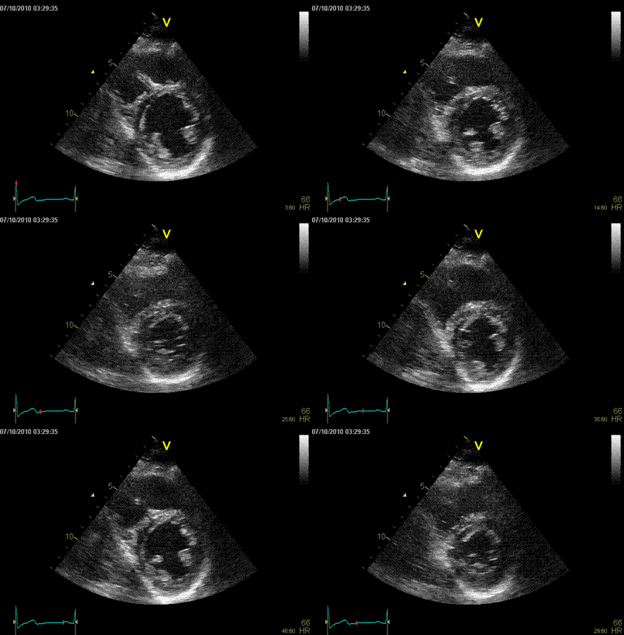


Normal ventricle in short axis view.
The loop can be used to generate an anatomical M-mode, the line is skewed to avoid the papillary muscles. On this M-mode the following values were measured: LVIDD: 53mm ,LVIDS: 36mm, giving a FS of 32%, IVDS 7 mm, IVSS 11mm, giving a wall thickening of 57%, LVPWD 8mm, LVPWS 11mm, giving a wall thickening of 38%, and a mean wall thickening of 48%.

Below are shown transmural strain by 2D strain with different ROI width. The images are all processed from the loop above, and endocardium traced in standard manner. In reprocessing, only ROI width was changed without changing the initial contour. All ROI's were accepted by the analysis software for all segments:
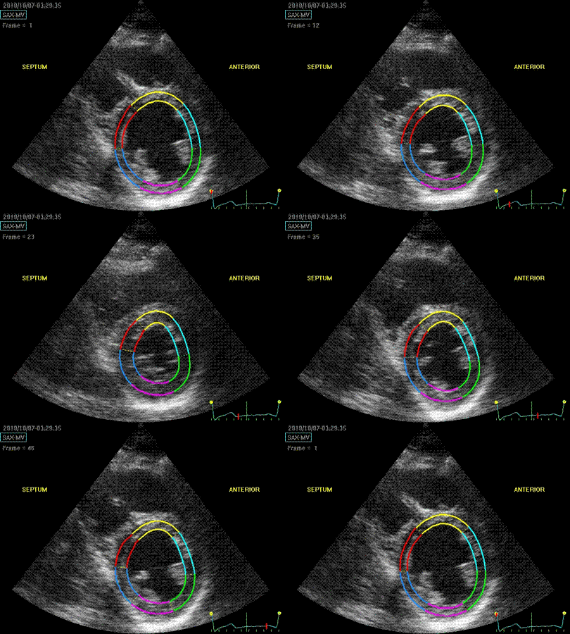


Transmural strain with narrow ROI setting. Tracking seems fair.  In the septum, tracking is good, but the relative wall thickening is absurd, 77 and 91!; normal  endocardial motion in absolute terms, gives a too high relative wall thickening in percent of the narrow ROI. Thanks to Ben Bulten of the Univerity of Twente, who pointed out that the image in this frame was erroneous.

Transmural strain with default (medium) ROI setting. Tracking seems fair.

Transmural strain with a wide ROI setting. Tracking seems fair.  Mean WT = 37%, because a normal endocardial motion in absolute terms will result in a low percentage of the too wide ROI.

The measured wall thickening is evidently as expected a function of diastolic ROI width, as expected. Compare also mean and the relevant segments with the values above

It is evident that the transmural strain is extremely sensitive to the ROI width. This is pertinent to long axis analysis also, as the curvature in the apical segments will lead to an increased susceptibility of the ROI width. This may be some of the reason why Becker et al (212) found transmural strain even in segments with total transmurality of scars, and not tethering as presumed.
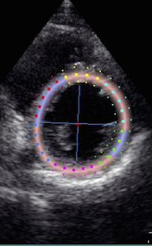


Cross section from the same loop, processed with a narrow (top) and wide (bottom ROI)
Radial strain values from the two different ROI's to the left, showing again a huge effect of ROI width on transmural strain values.
Circumferential strain from the same processings, the narrow sector gives a mean circumferential strain of -24.2%, the wide sector -29.2. Thus, the circumferential strain is more dependent on the depth of the measurement, than the width of the ROI.

Repeatability of 2D strain.

Basically, the 2D strain application, due to a high amount of smoothing, should have a high repeatability, as shown here. However, this will only be the case as long as the tracing is done in the same manner each time, in the same loops. This means a very standardised endocardial tracing, and a standardised ROI width. As shown above, the values are extrmely dependent on the ROI, both curvature and width of the ROI. Utilising the automated features of the application will ensure this, but will not necessarily ensure the correct shape and  width of the ROI, and hence, not necessarily the correct values either. In a study (208) where repeated measurements in the same loops was compared for different centres, the 95% limits of agreement were -11.4% to +11.8%, but with very little bias. Repeated recordings within one hour (presumably by the same observer), had limits of agreement of -9.6 to + 9.7%.


Both segmental strain and 2D strain have been compared for longitudinal strain, and compared to tissue Doppler (151, 153) as shown in this table. Both seem to agree fairly well. In addition variability of strain rate (but not strain) is lower by both methods than by tissue Doppler. However, both Segmental strain and 2D strain use automatic segmentation, this may be some of the reason for better repeatability, not speckle tracking vs. tissue Doppler per se. However, the higher variability of strain rate by velocity gradient, shows this method to have a somewhat higher noise componenet. Feasibility of both methods is reported to be between 70 and 80% of segments (lower in the HUNT study,but this is due to the aim of the study, to provide normal values as free as possible from artefacts.


Summary of differences and limitations of segmental speckle tracking and 2D strain.

It is important to be aware of the limitations of each method. It should also be emphasized that different methods are not necessarily directly comparable, and may yield different normal values and cut offs, due to the different ways parameters are measured. One of the fundamental differences stem from the different geometrical assumptions that are present as shown below:


Differences in geometry between methods. The fairly invariable outer LV contour is shown in heavy black. The diastolic inner contour, segmental borders, kernel positions and measurement lines are shown in light black. Systolic inner contour,
segmental borders, kernel positions and measurement lines are shown in red. Left: Segmental strain by tracking of kernels at segmental borders. It can be seen that the main deformation is measured along the longitudinal axis of each segment. As the wall thickens, the longitudinal mid line of the segments moves inwards, but in the basal and mid wall segments this does not add to the shortening as the angle does not change much. In the apex, however,  the angle of the center line changes,  contributing to the segmental shortening when it is measured by this method, however, the effect is slight.  To the right is shown the geometric assumptions of the 2D strain method.  The ROI uses an assumption of equal thickness from base to apex, and the mid line moves with the thickening of the contour.  The segment length is measured along the curved line, and both the curvature and the angle contributes to the shortening of the segment mid line as it moves inward. Thus, the shortening (strain)  might be expected to be higher in the apical segments by this method, as well as being dependent on the curvature, especially in the apex.  (However, this effect may be masked by the high degree of smoothing inherent in the application, which may distribute the differences between segments.  Ultrasound beams are shown in blue, illustrating the alignment problem of this method,  thus resulting in lower values in segments that are poorly aligned.


Inter vendor differences in speckle tracking

As speckle tracking have been attempted to be a solution to the shortcomings of tissue Doppler, and as this can be done in ordinary B-mode. most vendors have in time come up with speckle tracking applications in their analysis software. Also, vendor independent software, using the DICOM standard, are available.

This has been an interesting development, as the later studies have sbhown a fair amount of variability between strain measurements by different vendors (373 - 382). Normal values are not sufficiently harmonised that measures are interchangeable. For longitudinal 2D strain, biases of 1% absolute (373 - but here both methods had a much larger bias against MR tagging), to 5% (375).

and with correlations between measurements in same-day measures in the same patients vendor specific software as low as 0.35 (374) to 0.23 (377), but with no or less differences between different acquisitions when analysed in the same software (374), suggesting that the differences in software is the main source of variability between systems. However, even different versions of the same software has been shown to result in different measurement values (377). In general, variability have been found to be between 2 and 5% between software (378). It has been suggested that reproducibility is better than for EF measurements, but taking into account that EF by biplane tracings is the poorest reproducible parameter, this argument does not impress much.

Reproducibility within the frame of one software vendor, is much better, not surprising as discussed years ago in the paragraph above, the smoothing will always yield good repeatability (in fact, if you smooth the curves to zero, repeatability will be 100%), but still it has been found to be unacceptably high in newer studies, even within the frame of one software (377).

Although some researchers have found a fair correspondence between global strain measurements, (376), reproducibility of regional strain is much poorer.  Reproducibility is not better in 3D speckle tracking (379-383). Also, the 3D camp maintains that automated 3D volume and EF is far more reproducible, and thus the balance may tip away from 3D strain.

The variability is not especially surprising!

As discussed years ago, how the strain is defined has an impact on measurements especially the length of the wall. Curvature dependency of the ROI is also an issue, in a wide ROI, the inward motion (which is really circumferential shortening) will be interpreted as longitudinal strain. And this again is dependent how wide the ROI is defined in the apex.


This of course, not only affects the performance of different softwares, but also the repeatability, which in newer studies are much lower than previously reported (377), not surprising seeing the randomness of basic settings in ROI size and shape.


Of course, the number of speckles included in analysis, the definition of stability of speckles as this will define the amount of drift that is permitted by the software, and these are also specific to each. Finally, the amount and type of smoothing may vary.


The main limitation of any echo method is the ones related to data quality.

AS discussed under each method;
  • The fundamental limitations related to all methods are the ones arising from:
  • Tissue Doppler, having the advantage of high frame rate has additional limitations related to:
  • Speckle tracking (in any form), being less angle dependent has additional limitations relating to:
  • Segmental strain, being robust and giving the opportunity of utilising both tissue Doppler and speckle tracking and eliminating the angle problem, has the additional problem of:
  • The 2D strain application, being robust and user friendly, has the additional problems of:
    • Smoothing, relying heavily on AV-plane motion,
      • which may give strain values even where there are none, and may reduce sensitivity for reduced regional function
      • Makes the tracking more difficult to assess visually
    • Curvature dependency, due to the technicalities of the specific applications, which may give too high values in the apex.
    • ROI width seems to be critical, espacially in transmural strain.

How do the methods compare?


Going through a challenging case:


There is hypokinesia in the apicoseptal segment. The lateral wall seems to move fairly OK, almost to the apex. In addition, there is nearfield clutter, more pronounced in the lateral part, and a stationary reverberation in the lateral base.
Looking at peak values from the speckle tracking application in a bull's eye pliot, there is -18% strain in the apicoseptal segment, as well as -22% in the basal lateral. However, there is apparent hypokinesia in the apical and mid lateral wall.

However, as curve shapes generally gives more information, curves are given here:

There is an apparent hyperkinesia in the basal lateral wall, which is due to the segment being "squeezed" bwetween the mitral ring and the lateral wall. There are lower strains in the region of nearfield clutter, but also due to the reverberation, taking away the motion of the basal border of the mid segment. However the hypokinesia seems to have been smoothed away. This smoothing may also be influenced by the clutter regions.


Comparing with tissue Doppler derived curves, the pathological apicoseptal segment is clearly visible, both by curve shape, and values. The tissue Doppler is even more vulnerable to clutter, but as every ROI is processed separately, there is no carry over effect to segments with good image quality.


The same patholgy is visible in the apicoseptum by the time course in this M-mode, but it also serves to show how badly affected TDI is by the clutter in the lateral wall. However, timing of the main phases (Ejection, E, A, is still visible.


In large infarcts, they seem to give about the same information:

 
Pathology is evident, both in M-mode
And in strain / strain rate


Strain rate curved M-modes from tissue Doppler (left) and Speckle tracking (right). The speckle tracking image is much more smoothed, in time due to lower frame rate of B-mode compared to tissue Doppler. IN depth due to the spline smoothing of the 2D strain application. However, in this case, the resolution is sufficient to show intial stretch, apical hypokinesia and post systolic shortening also by 2D strain.


This can also be seen in strain rate curves, the magenta curve in the left panel and the cyan curve in the right panel are from the middle septal segment. The scales on the TVI and speckle tracking are not equal.


And in this case, the strain values do show the infarct, both  as curves, peak values and on the bull's eye map.

In this case, the infarct was rather large, and no method had any trouble in diagnosing it (nor has B-mode).

The next case is a small apical infarct:


Again, the SRI CAMM from speckle tracking has much less resolution both in time (due to lower frame rate) and space (due to smoothing). The apical hypokinesia cannot be seen, but the presence of initial stretch as well as post systolic shortening in the apex might be considered (but is far less evident than in TDI). Also in this case, the time course seems to give most information.


Here, the peak systolic strain in the apex of -14 and -15 is near normal, and the Bull's eye of peak values is not convincing either. There might be a slight discernible PSS in the two apical curves (green and cyan), but this is also within normal range. Time course in SR CAMM seems to be the best indicator.
TDI strain shows a peak systolic strain of -6, and evident PSS.

In this case both smoothing and curvature dependency might contribute to hide the apical dysfunction.


In case 6, the peak strain in the inferobasal segment is reduced, but might be interpreted as inaccurate processing when seen in the bull's eye view. The best clue to the infarct is the curve from the basal segment (yellow) showing reduced systolic strain and post systolic shortening, i.e. the time course, but in this case the hypokinesia is evident. And in this case both curves and values correspond with the two methods

In this case, the inferior infarct is visible. In another, nearly similar case, however, the infarct was not very visible in speckle tracking:


Strain by tissue Doppler, showing systolic akinesia in the basal segment (cyan curve) - mark how the ROI is placed to avoid the lower part of the segment where there is angle discrepancy), and normal strain in the apical segment (yellow) and the anterior wall (red). Strain by 2D strain, showing borderline reduced strain of -12% in the basal segment. In this case, the strain  is due to the inward motion (by tethering) which reduces the length of the curved segment. In addition, the ROI, being the same all the way around, overestimates the wall thickness in the infarct. In this case, the effect is due to the curvature, not smoothing.


Finally where there are drop outs, the spline smoothing may distribute the motion over fewer segments, thus masking the infarct totally:


Stiff inferior wall due to an infarct, but fair annulus motion due to normal, or even hyperkinetic apical segments.


-  which results in the normal annulus motion being splined over only three segments, instead of six, as there is a drop out of the whole anterior wall, and the segments are excluded, as opposed to TDI where analysis is only local.


Back to main website index.

References:


Editor: Asbjørn Støylen Contact address: asbjorn.stoylen@ntnu.no


b