This section extends the basic concept of strain into the specific
geometry of the left ventricle. It is important to understand that
strain is about changes in myocardial dimensions. Thus strains the
components of myocardial volume changes, and only expressions of
geometry. The effects seen by strain rate imaging is thus explained
by geometry, not by material prpoperties of the myocardium, over all
geometry governs the changes and relations between strain
components. This is true of all strains, longitudinal, transmural
and circumferential as well as area strain. Also, the strain
gradient across the wall seen both in transmural and circumferential strain is due to geometry,
not differential fibre action.
Still preaching my
personal litany: Strain is geometry.
(Cormorant, Galway, Ireland).
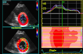
Normal strains,
longitudinal, transmural, circumferential. There is
systolic longitudinal shortening, circumferential
shortening and transmural thickening.
The strain components are simply coordinates of the three
dimensional deformation of the myocardium, and has nothing to do
with material properties of the myocardium, such as anisotropy or
fibre directions in a direct sense. Of course, the total deformation
is a function of fibre shortening, and ultimately, among other
things fibre architecture, but also of load and valve function. And
it is of note, that while systolic deformation deformation continues
to end ejection, myocardial relaxation starts at peak pressure.
ContractilityBasically, strain is the total systolic shortening,
equivalent to the isotonic shortening in experimental models,
and thus very afterload dependent. Peak systolic Strain rate,
on the other hand has been shown to be more closely related to
contractility, but the physiological limits of this
correlation is discussed.
Stroke
volume It has been shown that strain relates best
to the stroke volume, and thus is both afterload and volume
dependent.
Timing
Strain rate, being the temporal derivative of strain shows
more detectable shifts, especially in colour M-mode, making it
more useful for timing purposes.
Normal
left ventricular dimensions Left ventricular
dimensions and geometry is closely related to the geometry of
left ventricular strain. Thus, normal values and the relation to
body size, age and gender are included here. Normal values
provided from the HUNT study.The data from the HUNT study suggests thatrelative wall thickness are both body size and age
dependent, that while wall
thickness increases with age, LV length decreases, invalidating
previously findings of M-mode based LV mass increase with age.
Finally, the ratio
of LV length and external diameter is BSA
independent and (nearly) gender independent, but decreases
with age, being a measure of age related remodeling. Tables of
normal findings from the HUNT study are added.
LV
volumes and age. Due to the simultaneous increase in
wall thickness and decrease in length, there is no increase
in LV volume by age, when the age dependent increase in BP
is considered.
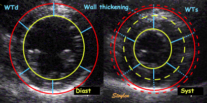
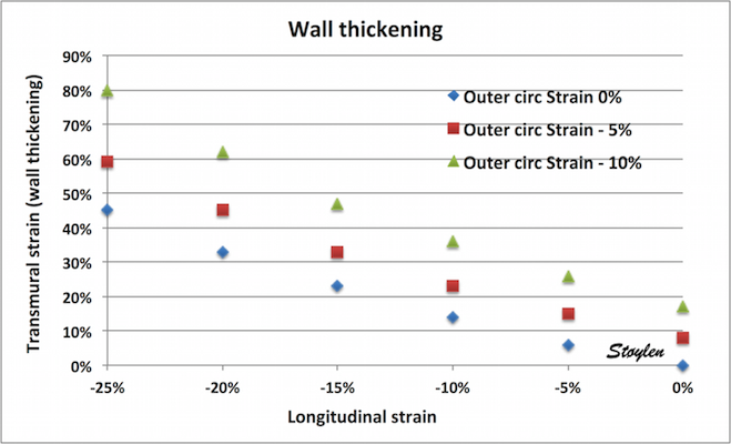
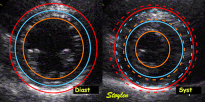
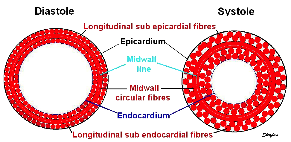
Speckle tracking strain tracks not only wall shortening,
but also wall thicening. And as the wall thickens, both
the midwall and the endocardial (even more) alyers moves
inwards. This inward motion will in itself make the lines
shorter, which is an additional effect to the true wall
shortening. Thus Speckle tracking strains overestimates
true wall shortening.
There
is no gold standard for Global longitudinal strain.
As there is no universal algorithm for global
strain, of course the concept of global strain as a universal
measure of ventricular function has no exact meaning. It is
only a theoretical concept.
This means there is no reference standard, they are method
dependent. This means that strain values cannot be validated,
and different methods cannot be compared in terms of validity,
and finally, normal values do only have validity within the
method used.
There is no universal definition, and thus no "ground truth"
at all for GLS. Methods cannot be validated, and GLS has to be
considered only within the method used.
Normal
transmural gradient of longitudinal strain The
gradient in longitudinal strain seen by speckle tracking
methods, can simply be explained by the speckle tracking,
the inward motion is most pronounced at the endocardial
surface, less at the midwall, and least at the outer
surface. This apparent shortening is not true shortening,
but a systematic error due to tracking of wall thickening,
and can explain the gradient of longitudinal strain.
Even though analysis software will produce layer values
at request, layer strain separation depends on line
density, line width, direction in relation to the wall (in
order to avoid pericardial echoes), and focussing. Number
of lines is again dependent on frame rate. It is difficult
to achieve a sufficient line density as well as narrow
enough lines.
Transmural strain which some calls "radial strain". The
term "radial, however, is ambiguous, as in general
ultrasound terminology this means "in the direction of the
ultrasound beam".There is no such thing as "radial
function". Radial strain means wall thickening, but there
are no myocardial fibres going in the radial direction. Wall
thickening is a function of wall shortening, and
circumferential shortening.
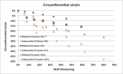
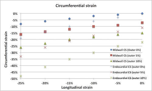
Circumferential
strain Circumferential strain do NOT
reflect circumferential fibre contraction. There would have
been circumferential shortening even without circumferential
fibres. Circumferential strain is mainly the circumferential
shortening due to inward movement of midwall or endocardial
circumference as the wall thickens. As different vendors use
different definition of circumferential strain (midwall or
endocardial), there is no standard circumferential strain.
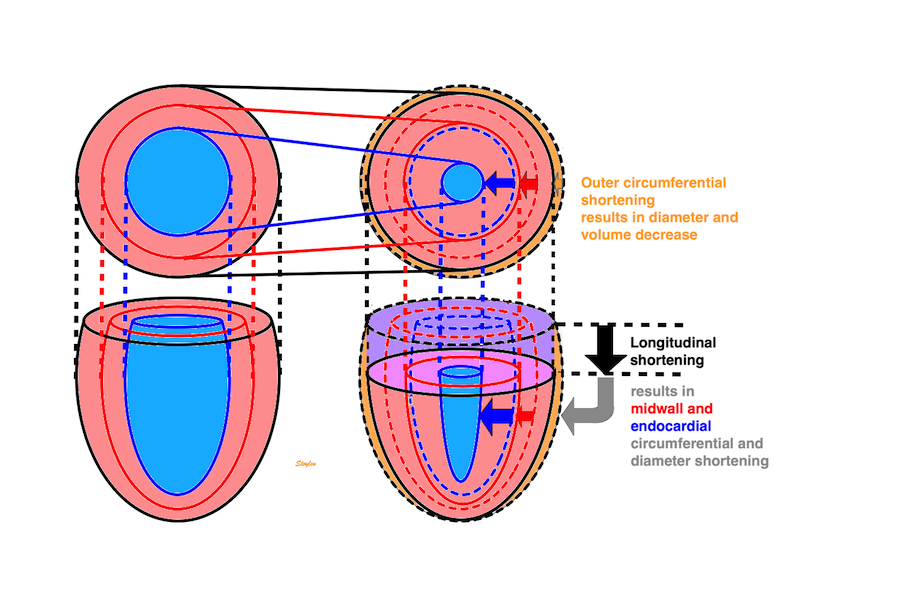
Inter
relations of all three major strain components
As the myocardium is nearly incompressible, the three
strains must be interrrelated. Longitudinal shortening will
give transmural thickening, and transmural thickening
(inwards) will give inward motion of endocardial and midwall
circumferences. In addition, there is a small outer
circumferential shortening, so all thickening occurs
inwards. This is the cause of the inwards gradient of
transmural and circumferential strain.
Incompressibility
and the myocardial strain tensor there is
no gold standard for strain, and different sets of assumptions
as well as specific methods will give different values. This
also means that both the inter relations of strains, as well
as the relations to the myocardial volumes and
incompressibility calculations will vary, and at the present
level of technology, strains cannot be used to decide if the
myocardium is incompressible.
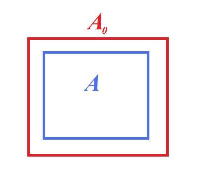
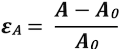
Area strainArea
strain is neither the sum, nor the product of
circumferential strain. A slightly simplified modelling
will give the formula A = L * C + L + C . Thus, area
strain is a function of longitudinal and circumferential
strain, not a "new" parameter.As different vendors use
different definition of area strain (midwall or
endocardial), there is no standard circumferential strain.
MAPSE
contribution to the stroke volume: MAPSE
contributes about 75% to the total SV (although this is
not normative as the geometrical model has limitations.
However, while MAPSE decreases with age, there is no
compensatory increase in short axis function (which
actually also declines), to explain maintained EF. EF is
maintained with increasing age by the simultaneous
decrease in LVEDV and SV, keeping the ratio constant.
Also, MAPSE remains a constant percentage of the
decreasing SV. The notion that circumferential function is
the main contributor to SV, is bases on the lack of
uncerstanding that circumferential strain (except external
CS) is partly due to wall thickening, which again is
mainly due to longitudinal shortening.
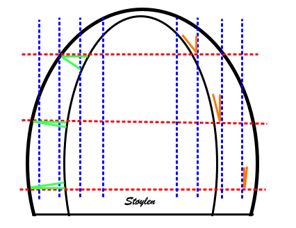
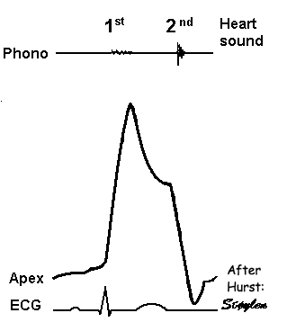
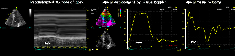
As the apex is stationary, while the base moves, the displacement
and velocity has to increase from the apex to base as shown below.
As the apex is stationary,
while the base moves toward the apex in systole, away
from the apex in diastole, the ventricle has to show
differential motion, between zero at the apex and
maximum at the base. Longitudinal strain will be
negative (shortening) during systole and positive
(lengthening) during diastole (if calculated from end
systole).
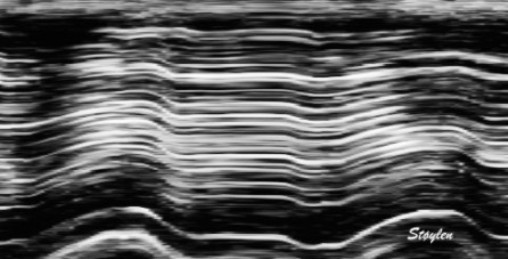
M-mode lines from an M-mode
along the septum of a normal individual. These lines
show regional motion. It is evident that there is most
motion in the base, least in the apex. Thus, the lines
converge in systole, diverge in diastole, showing
differential motion, a motion gradient that is equal to
the deformation (strain).This difference in
displacement from base to apex is also evident in the
displacement image shown above.
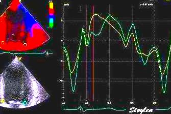
Velocity gradient
AS motion decreases from apex
to base, velocities has to as well. Thus, there is a
velocity gradient from apex to base, which equals
deformation rate.
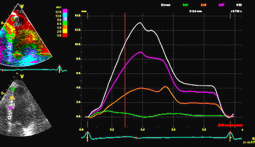
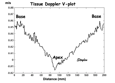
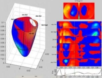
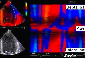
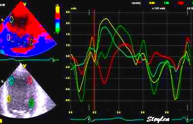
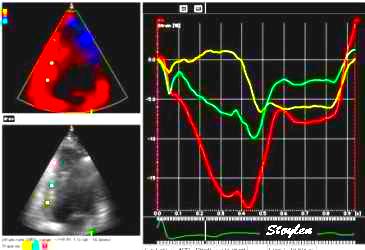
Spatial distribution of
systolic velocities as extracted by autocorrelation.
This kind of plot is caled a V-plot (247).
It may be usefiul to show some of the aspects of strain
rate imaging. The plot shows the walls with septal base
to the left, apex in the middle and lateral wall base to
the right. As it can be seen again the velocities are
decreasing from base to apex in both walls. There is
some noise resulting in variation from point to point,
but the over all effect is a more or less linear
decrease. The slope of the decrease equels the velocity
gradient. (Image courtesy of E Sagberg). However, this
shows only one point in time, and all values are
simultaneous.
Thus there is a velocity gradient in systolic velocities, from base
to apex. This is equal to strain rate. In fact, the strain rate is
displayed by the slope of the V-plot.
However, the V-plot is the instantaneous
velocity gradient, which may differ from the peak strain rate,
if peaks are at different times in different parts of the
ventricle.
Strain rate is calculated at the velocity difference per length
unit /velocity gradient) between two points in the myocardium:
The velocity difference varies during the heart cycle,
and the distances are shaded red when the differences are
negative (v1<v2), and blue when they are positive
(v1>v2). The resulting strain rate curve is shown to the
left, with negative strain rate shown in red, positive shown
in blue. Mark also that the peak strain rate and peak
velocities are not simultaneous in this segment.
This is shown in more detail here. Peak velocity (left,
A) is earlier than peak strain rate (Middle, B), but from the
figurte to the right, it is shown that B is the point of
maximum ditansce between the curves.
Thus the distances between the two curves is an
indication of the strain rate:
Left: velocity curves. Middle: strain rate curves from
the two segments between the velocity curves. Right, the areas
between the velocity curves corresponding to, and shaded with
the corresponding strain rate curves. Peak strain rate is not
simultaneous in the two segments, peak velocity is more
simultaneous due to the tethering effects. This is described
in more detail here.
But this means that the global strain rate (of a wall or the whole
ventricle), equals the normalised, inverse value of the annular
velocity:
Diagram showing that for the whole ventricle,
v(x) is apical velocity = 0, and v(x+x) = S', then SR = -S'/WL
If the two
points are at the apex and the mitral ring, the apical
velocity , apex being stationary, and is
annular velocity. then
equals wall length (WL), thus and
peak .
Thus, peak strain rate is peak annular velocity normalised for
wall length.
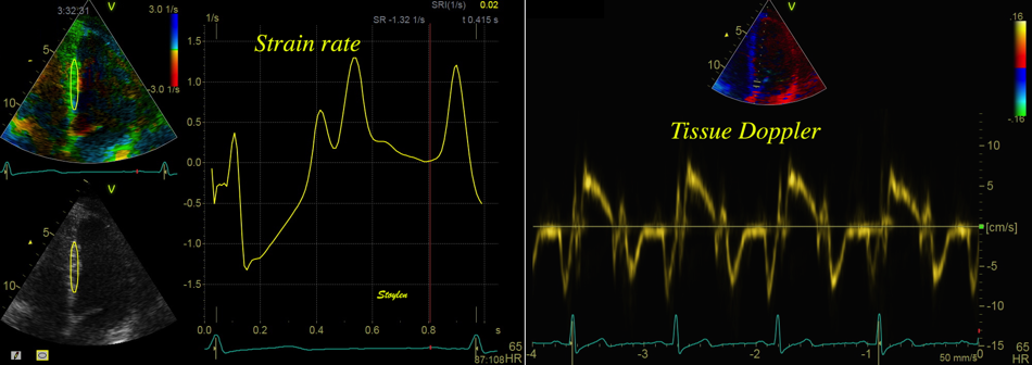
Comparison between velocity and strain rate. Left, strain
rate of most of the length of the septum, right spectral Doppler
of the mitral annulus of the same wall. The two curves can be
seen to be very similar, although the strain rate curve is
inverted as explained above. Also, the values and units are
different, as strain rate is divided by the ventricular wall
length. The summed strainrate curve has peak strain rate very
close to the time of peak velocity, but tihis is due to the
averaging effect, as peak strain rates differ between segments.
Exactly the same is the case for basal displacement vs strain, of
course as shown in the basic concepts section.:
The difference in displacement varies during the heart
cycle, and the distances are shaded red, always being negative
(d1<d2). The resulting strain curve is shown to the left,
strain rate being negative during the whole heart cycle,
isshown in red. Mark that as opposed to peak strain rate and
peak velocities, peak displacement and peak strain are
simultaneous, being near end ejection.
Strain rate and strain assessed by offset between velocity
curves
Strain rate and strain can be visually assessed by the
offset between the curves, when the velocity curves are
obtained from points with a known (and equal) distance.
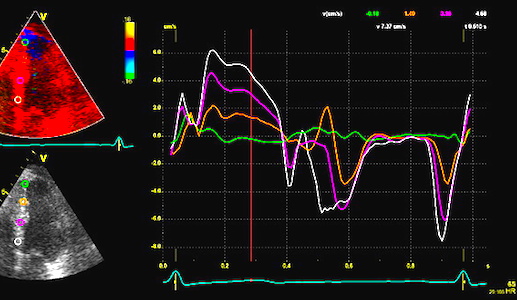
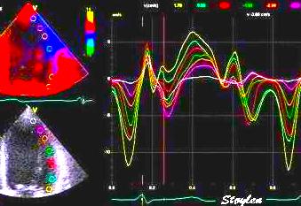
Segmental strain rate from
velocities: Velocity curves
from four different points of the septum. The
image shows the decreasing velocities from base to
apex. The distances between the curves show the
strain rate of each space between the measurement
points (segments).
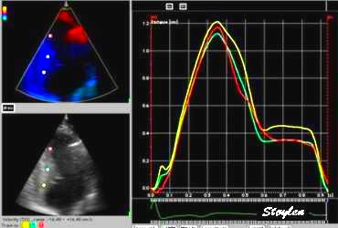
Segmental strain from
displacement. Displacement curves from the same
four different points of the septum, obtained by
integration of the velocity curves. The
image shows decreasing displacement from base to
apex. The distances between
the curves show the strain
of each space between the measurement points
(segments).
If the curves are taken from the segment
borders, this is a representation of the segmental strain
rate and strain. Thus, it is evident that the strain rate
and strain can be visualised (qualitatively) by the spacing
of the velocity
and displacement curves, even without doing the
derivation.
Thus, basal velocities are equivalent to wall strain rate, and
basal displacement, are equivalent to wall strain:
Septal strain and strain rate (right) from (nearly) the
whole septum, and basal septal velocity and displacement
(left). As the apex is (nearly) stationary, the basal velocity
and displacement is a motion inscribing the whole of the
shortening of the wall, the deformation curves from of the
whole wall is very near the inverted motion curves from the
base as described elsewhere.
The negative deformation curves is from the original
Lagrangian definition where shortening is baseline
length + resulting length, becoming negative when there is
shortening. Motion measures are absolute, deformation
measures are relative. Peak shortening can be measured as
either peaks systolic annular displacement (MAPSE) and peak
systolic strain, and shortening rate as peak systolic basal
velocity, the S' or peak systolic strain rate, SR. All four
measures are in clinical use with ultrasound.
The strain rate being the difference between the decreasing
velocities from base to apex, means that
Is there an apex to base
gradient in strain and strain rate as well?
It has been maintained that as the curvature is larger (smaller
radius both in cross sectional and longitudinal planes) in the
apex, the wall stress (i.e. load) is lower, and hence shortening
higher, in accordance with the law
of Laplace. However, this reasoning do not take the varying
wall thickness into account. As the wall is thickest at the base,
and thinnest at the apex (62),
the wall thickness decreases as the radius decreases, and no
conjectures about the wall stress can be made.
As apex is stationary, and the base of the ventricle moves, there
has to be a gradient in velocity and motion from base to apex. As
strain rate actually is that velocity gradient, the presence
of a gradient in strain rate depends on whether the velocity
gradient is constant or not. Looking at the V-plot,
the curve seems fairly straight, i.e. the velocity gradient seems
fairly constant along the wall, indicating that there is no
gradient in strain rate.
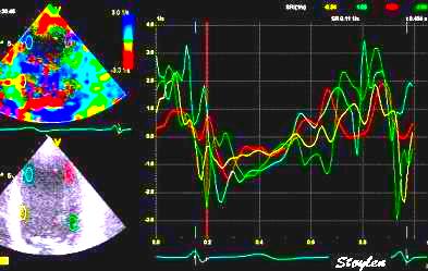
Good quality V-plot of
venlocities from
the septal base to the left through the apex in
the middle to the lateral base to the lateral base
to the right, shows
velocities as near straight lines, and
thus, a constant velocity gradient. This should
mean that there is no strain rate gradient from base to
apex.
A nearly straight line. Blue eyed
shags (cormorants) at Cabo de Hornos (Cape Horn), Chile.
Thus, while velocities decrease, strain rate seems more or
less constant from base to apex as described above. By reasoning
this should also apply to strain.
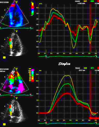
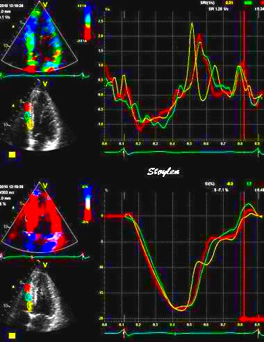
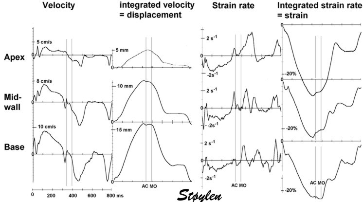
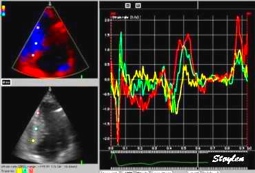
Motion (velocity and
displacement - left) and deformation (strain rate and
strain - right) traces from the base, midwall and apex
of the septum in the same heart cycle. It is evident
that there is highest motion in the base (yellow
traces), and least near the apex (red trace), and this
is seen both in velocity (top - actually both in
systolic and diastolic velocity) and systolic
displacement (bottom). The distance between the curves
are a direct visualization of strain rate and strain, showing fairly
equal width of the intervals. Strain rate (top and
strain (bottom) curves are shown to the left, showing no
difference in systolic strain rate or strain between the
three levels.
Some of the earliest strain rate studies found no
base - to apex gradient (10,
19,
341),
although later studies seem to find differences with lowest values in the apex (124). However,
in that study, the greatest angle
error was also in the apex (206).
This angle deviation , however may not be consistent, as discussed
here.
In the comparative
study between methods in HUNT (153),
(N=50)
using tissue Doppler velocity gradient, there was
lower values in the apex, but only only when the
ROI did not track the myocardial motion through the heart cycle.
Tracking the ROI eliminated this gradient, indicating that this
was artificial.
Velocity gradient
(stationary ROI)
Dynamic velocity
gradient (tracked ROI)
Peak Strain rate
End systolic Strain
Peak Strain rate
End systolic Strain
Apical
-1.46
(0.85)
-14.6
(9.0)
-1.31
(0.73)
-17.2
(9.1)
Midwall
-1.29
(0.56)
-18.2
(7.4)
-1.40
(0.58)
-16.9
(7.1)
Basal
-1.71
(0.94)
-19.6
(9.3)
-1.59
(0.74)
-17.1
(8.6)
Mean
-1.45
(0.79)
-17.7
(8.5)
-1.43
(0.67)
-16.7
(8.1)
Comparison
between standard tissue Doppler velocity gradient and tracked
ROI. Standard deviations in parentheses.
Thus, it seems fairly reasonable to conclude that the finding of
lower gradient in the apex is artificial.
But it may indicate that the negative base-to apex gradient, or
the lack of a positive gradient, may be a finding specific to
tissue Doppler derived strain.
Results from the HUNT study
(153)
with normal values based on 1266 healthy individuals. Values are
mean values (SD in parentheses). Differences between walls
are small, and may be due to tracking or angular problems.
No systematic gradient from apex to base was found.
This method tracks segmental strain by the segment endpoints,
longitudinal by tissue Doppler, and crosswise by speckle tracking,
thus a more angle independent method.
With 2D
strain, some authors have found a reverse gradient of
systolic strain as well, highest in the apex (mean 20.2%), lowest
in the base (mean 17.0%) (207),
a later study also found a gradient, but with higher values (18.3
bsally vs 23.0 apically) (423).
However, in that application, measurements are curvature
dependent, the curvature being highest in the apex and
lowest in the base, and the discrepancy between ROI width and
myocardial thickness being greatest.
Curvature
dependency of strain in 2D strain by speckle tracking. The two images are processed from
the same loop, to the right, care was taken to straighten
out the ROI before processing, while the left was using the
default ROI. In both analyses the application accepted all
segments. It can be seen that the apical strain values are
far higher in the right than in the left image (27 and 21%
vs 19 and 17%). However, the curvature of the ROI even
affects the global
strain, as also discussed above in the basic
section.
In the subset of 50 analysed for comparison
of the methods, taking care to avoid both foreshortened
images and excessive curvature, there were no level differences
in 2D strain either:
Segment length by
TDI and ST
2D strain (AFI)
Peak Strain rate
End systolic Strain
Peak Strain rate
End systolic Strain
Apical
-1.12
(0.27)
-18.0
(3.6)
-1.12
(0.37)
-18.7
(6.6)
Midwall
-1.08
(0.22)
-17.2
(3.2)
-0.99
(0.23)
-18.3
(4.7)
Basal
-1.03
(0.24)
-17.2
(3.5)
-1.12
(0.36)
-18.0
(6.2)
Mean
-1.08
(0.25
-17.4
(3.4)
-1.07
(0.33)
-18.4
(5.9)
Comparison between methods.
Standard deviations in parentheses.
In this case care was taken to align ROI
shapes as much as possible.
A large meta analysis of speckle tracking derived strain (427),
did not address this question.
Interestingly, a recent study looking at aortic stenosis, fond
that there was an apex to base gradient in the most severe cases
(reduced in the base), but no gradient in the less
pronounced cases (15.7 vs 16.3%) (418).
This, by corollary, should also be a case for no gradient in the
normal state. An even more pronounced finding is described in a
study of apical sparing(419), where the base to apex gradient (due to reduced strain
in the base was shown as a sign of amyloidosis (11.1 vs 18.1%), as
opposed to no gradient in the two reference populations: Normals
(18.7 vs 15.8%) and hypertensive controls as a hypertrophic
reference group without amyloidosis (16.4 vs 14.1%). It is notable
that in this setting showing the gradient
as a criterion for amyloidosis, the two
reference groups actually shows an inverted
gradient.
Thus, the base to apex
gradient may be a result of the speckle tracking software
combined with the processing.
MR studies have also found various results. Bogaert and Rademakers (171)
in a study of healthy subjects (N=87) found lowest longitudinal
strain in the midwall segments, higher in both base and apex,
but no systematic gradient from base to apex. Moore et al (384)
in a study of healthy volunteers (N= 31) found a systematic
gradient, but with the lowest strain in the apex, highest in
the base.Venkatesh
et al in a healthy subset from the MESA study (N= 129) (385)
examined only transmural and circumferential strains in cross
sectional planes, and found decreasing transmural strains from
base to apex in all layers. As segmental shortening and
thickening are very closely
related through incompressibility,
this should amount to a decreasing strain from base to apex too.
Circumferential strains, on the other hand, seemed to be less
systematic, and the apex to base gradient varied between both
layers and walls. This, however, is counterintuitive, as wall
thickening causes inwards displacement of the circumference,
wall thickening is equivalent to shortening, as the findings
should show the same gradient.
MR measurements have processing issues as well. Using short axis
planes, the planes will show an increasing deviation from the
90° angle with the wall, towards apex, causing an over
estimation of wall thickness in the apical planes. Using
magnetic tagging, this is usually done in a grid with 90°
angles, at least in the transverse/longitudinal direction, while
the radial might vary, although usually at 90° with the
horisontal plane. This might cause angle deviations as shown
below.
Diagram illustrating MR planes and magnetig tagging
grids and relation to myocardial directions. Horizontal planes
and grud lines (red) are usually cross sectional, causing
increasing angulation with the transverse direction of the
wall (green) towards the apex. Longitudinal grid lines deviate
increasingly from the longitudinal direction of the wall
toward the apex as well (orange).
A small study comparing both 2D strain, segmental speckle
tracking, segmental strain by the combined
method and velocity gradient by tracked ROI, all
in the NTNU software, did show the following results in 11
healthy subjects:
2D strain
Segmental ST
Segmental combined
Tissue Doppler
MRI tagging
Apical
-20% (3)
-18% (4)
18% (3)
18% (5)
-20% (5)
Midwall
-21% (2)
-20% (3)
19% (3)
21% (6)
-18% (4)
Basal
-20% (3)
-18% (4)
18% (4)
16% (6)
-18% (4)
(Standard deviations in
parentheses)
Thus not very much indication of such a gradient in any method.
Edvardsen, in a validation study (9)
of tissue Doppler derived strain vs. MR found 18.5% in the base vs
18.75% in the apex with tissue Doppler and 17.5 vs 18.25 with MR.
MR tagging may include algortihms for calculation of the local
coordinates, but this again will introduce new uncertainties in
the angle calculations, causing both over- and under corrections
depending on the calculation. Shear
strain may affect the motion of tags, and attempts to
calculate shear strains and separate them from the normal strains,
will again increase the complexity of calculations and possible
uncertainties.
Looking back to the animal
experiments with ultrasonomicrometry, Urheim (8)
found 12% in the base and 16% near apex under baseline
conditions. Korinek et al (428)
found 15.8% in the mid posterior segments vs 13.1% in the apical
segment under baseline with chrystals, and 11.9 vs 13.7 with 2D
strain. However, ultrasonic chrustal measurements are also
subject to geomatreic distortion, especially when placing the
chrystals in the sub endocardium, they will follow the inward
movement. In straight segments, (basally), this will not result
in shortening, but in curved segments (apically) this will lead
to an apparent segmental shortening, which will come in addition
to the true longitudinal shortening of the segment. This is
illustrated below:
Simplified image illustrating the
effect of inward motion (due to wall thickening) on a
pair of sub endocardial crystals close to the base and
close to the apex, respectively. The longitudinal
shortening, and thus true segmental shortening is
omitted. Blue: end diastole, Red: end systole. In the
base, the crystals are aligned with the wall, and the
inward motion simply displaces the crystal pair, with
no reduction of the distance between them. In the
apex, the crystals are placed on a curved surface. The
inward motion is thus also a reduction in the
curvature radius, and thus the crystals converge
(dotted black lines). This reduces the distance
between them, resulting measurement of an apparent
shortening of the segment, which the is added to the
true segmental shortening.
Illustration of this convergence
on measured segment shortening. In this image, similar
systolic segment shortening is shown. The convergence
in the apex due to the convergence is shown in red.
Without this convergence (using parallels - green),
would result in true segmental shortening, which is
less in the apex, more similar to the base.
Thus, the presence of a real
base to apex gradient in deformation parameters has so far
not been established.
Differences
between walls
Although Höglund did not find any difference in systolic mitral
annular displacement between different walls (30),
other
authors have found such differences, with lateral displacement
higher than the septal (167).
In
the large HUNT study, the same differences were found in systolic
annular velocities (165),
with
differences between septum and lateral wall was of the order of
10%, but not in deformation parameters (153),
where
the same difference was on the order of 4% in strain rate and only
1% (relative) in strain.
Normal annular velocities, strain rate and strain per wall in
the HUNT study. (From 153
and 165)
Anteroseptal
Anterior
(Antero-)lateral
Inferolateral
Inferior
(Infero-)septal
PwTDI S'
(cm/s)
8.3
(1.9)
8.8
(1.8)
8.6
(1.4)
8.0
(1.2)
cTDI S'
(cm/s)
6.5
(1.4)
7.0
(1.8)
6.9
(1.4)
6.3
(1.2)
SR (s-1)
-0.99
(0.27)
-1.02
(0.28)
-1.05
(0.28)
-1.07
(0.27)
-1.03
(0.26)
-1.01
(0.25)
Strain
(%)
-16.0
(4.1)
-16.8
(4.3)
-16.6
(4.1)
-16.5
(4.1)
-17.0
(4.0)
-16.8
(4.0)
Results from the HUNT
study (153,
165)
with normal values based on 1266 healthy individuals. Values
are mean values (SD in parentheses). Velocities are
taken from the four points on the mitral annulus in four
chamber and two chamber views, while deformation parameters
are measured in 16 segments, and averaged per wall. The
differences between walls are seen to be smaller in
deformation parameters than in motion parameters, although
still significant due to the large numbers.
This is illustrated below.
M-modes from the septal an
lateral mitral ring, showing that systolic
displacement is higher septally.
Pw tissue Doppler from the septal
and lateral mitral ring, showing the lateral peak
systolic velocities to be highest.
As this is not the case for strain
and strain rate, this is illustrated below:
Colour Doppler from the four chamber view, traces
from the septum (yellow) and lateral wall (cyan). In this
image, the peak velocity and displacement shows bigger
differences than peak strain rate and strain
Tethering
The velocity gradient is closely related to the concept of
tethering, which means that a myocardial segment may move due to
being tethered to a neighboring segment. This means, that as the
apex is stationary, the apical segments have no motion due to
tethering, but only intrinsic deformation (shortening). However, the
shortening of the apical segments will move the midwall segments,
and would have done so, even if they were passive. In a normal
myocardium however, they also have normal deformation (shortening).
This, of course, means that they have both motion due to tethering,
as well as intrinsic deformation. They will then transmit their own
passive motion component to the basal segments, as well as imparting
motion by their own contraction, making the basal segments move more
and faster. And the basal segments shortening as well, will make the
annulus move fastest and most of all.
The systolic motion of each myocardial segment from the apex to the
base is the result of the segment's own deformation, added to the
motion that is due to the shortening of all segments apical to it.
Thus, as the apical segments shortens, this segment will pull on the
midwall and basal segments ( this is passive motion - tethering),
the midwall segment also shortens, and pulls even more on the basal
segment, which is shortening as well. As the apical parts of
the ventricle pulls on the basal, the displacement and velocity
increases from apex to base (25).
This means that some of the motion in the base is an effect of the
apical contraction - tethering.
In fact, completely passive segments can show motion due to
tethering, but without deformation. (4,
6,
7).
This means that the velocity (and displacement) are position
dependent, while strain rate (and strain) are much more position
independent, if the velocity gradient is evenly distributed.
This is illustrated below.
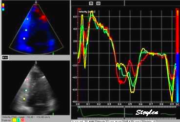
Velocity,
displacement, strain rate and strain from three
different points, apex, midwall and base, in the septum
of a normal person. These curves all represent the same
data set. It is evident that motion (velocity and
deformation) increases from apex to base, showing a
gradient, while deformation (strain rate and strain) is
more constant, in fact a direct measure of the motion
gradient. Diastolic deformation is far
more complex, and is discussed below.
Motion (velocity and
displacement - left) and deformation (strain rate and strain -
right) traces from the base, midwall and apex of the septum in
the same heart cycle. It is evident that there is highest motion
in the base (yellow traces), and least near the apex (red
trace), and this is seen both in velocity (top - actually both
in systolic and diastolic velocity) and displacement (bottom). The distance between the curves are a
direct visualization of strain rate and strain, showing fairly equal
width of the intervals. Strain rate (top and strain (bottom)
curves are shown to the left, showing no difference in systolic
strain rate or strain between the three levels.
The point of tethering it that a passive segment is tethered to an
active segment, and thus is being pulled along by the active
segment, without intrinsic activity in the passive segment. This
means that a passive segment may show motion, but without intrinsic
deformation, and the deformation imaging will discern. This is
evident both in systole and diastole. tethering
effects may show diverse results. It has three important
consequences:
Infarcted segments may be totally akinetic, but still being
pulled along by active segments, showing motion without
deformation. In this case, no offset between displacement
curves, means no strain. This is usually evident in the inferior
wall. A perfect example of a totally passive, tethered segment
moving close to normally, can be seen below, and in more detail
here.
It may also be pertinent to the basal part of the right
ventricle. In both cases, the annular motion may be near to
normal due to hyperkinesia in the neighboring segment, as this
segment is offloaded as explained here.
Tethering: The
basal and midwall segments are infarcted, and are
being pulled along by the active apical segment. The
whole inferior wall seems stiff.
The
stiffness is evident in velocity and displacement
curves. All of the wall has motion, which must be due
to the apical segment, but as all curves lie on top of
each other, the whole wall moves as a stiff object,
i.e. there is no deformation below the apical point,
and thus akinesia.
Strain rate and strain
curves, however, show that the findings are more
differentiated, showing akinesia basally (yellow),
hypokinesia in the middle (cyan) and hyperkinesia in
the apex (red).
Thus; in this case, the passive segment is
tethered, showing motion and masking the pathology to some
degree. Deformation imaging will show this.
If there is pathological contraction at some time in the heart
cycle (e.g. post systolic shortening), the shortening of a
pathological segment may impart motion to a whole wall.
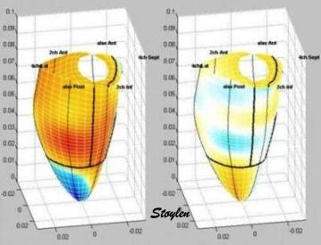
Velocity images showing
motion towards the apex in red, away from apex
in blue. Left, systolic 3D reconstructed
image, showing normal motion in the septum and
inferior wall, and paradoxical motion in the
inferolateral, lateral and anterior wall. Right, o
top are bull's eye from systole, showing the same,
as well as early diastole showing inverse motion
during the e-phase, i. e motion of the whole wall
towards the apex in diastole. Apparently, the whole
anterolateral half of the ventricle is ischemic .
Strain rate images from
the same recording, left systole, right early
diastole, showing that the ischemia is due to a
smaller ischemic area in the inferolateral, lateral
and anterior apex, where there is stretching during
systole (blue). This stretching, results in
the midwall and basal segments moving away from the
apex, despite contracting normally. In early
diastole there is recoil in the ischemic area
(yellow), resulting in anterior diastolic motion in
the whole of the wall. In this case, the
ischemia is obviously limited to a part of the apex,
the rest of the motion abnormalities being due to
tethering.
In this case, the normal segments in the midwall and
base of the affected wall has abnormal motion due to being tethered to the pathological
segments in the apex.Another, similar example of this in ischemia, can be seen
below. Thus, it may mistakenly be taken ass asynchrony
between walls. Deformation imaging shows the true location and extent of
the pathology. In phases where parts of the myocardium is active, other
passive, due to differences in timing, the tethering of passive to
active segments may make the whole myocardium move throughout the
whole phase, even if each segment is active only part of the time.
This is evident in diastole, where elongation occurs at different
times in the different levels of the myocardium.
Translational effects:
Overall motion of the heart will reflect in each and every segment
the translational motion added to the local measurement.
In this video the rocking
motion of the left ventricle is evident, the whole heart
rocks toward the left in systole. (However, this is NOT
due to conduction delay).
However, looking at
deformation (wall thickening - transmural strain) in
this cross sectional recording, the wall thickening can
be seen to be normal and symmetric in both onset and
extent.
In fact, wall thickening in the cross section seems to supplement
the impression from the four chamber view, that the rocking motion
is not regional dyssynergy. Wall thickening is transmural strain.
Apparent
asynchrony: Looking at mitral valve velocities, the
lateral wall (cyan) seems to have a delayed contraction
compared to the septum (yellow), both looking at onset
and peak velocities, indicating either asynchronous
activation or initial akinesia of the septum
Looking
at multiple sites in the lateral wall, it seems that the
delay in early ejection phase corresponds to positive
velocity in the base (yellow), zero velocity a little
more apical (cyan), and increasingly negative velocities
toward the apex, i.e. possible apical initial dyskinesia
(which might be ischemia).
The
curved M-mode from the base of the septum through the
apex to the base of the lateral wall shows the same
effect, normal timing of the velocities in the septum,
inverted velocities in the apical two thirds of the
lateral wall.
Comparing tissue velocity
with strain rate in the base and apex, however, , we see
that the apparent delayed motion in the lateral wall has
no corresponding delay in deformation, wheteher looking
at onset of, or peak negative strain rate. All
four parts shortens synchronously and normally. Thus, it
illustrates that the rocking motion velocities are added
to the velocities, the subtraction algorithm of the velocity
gradient subtracts these velocities again, showing
the true timing of regional deformation.
In this case, the motion (velocity imaging) is mis informing, giving
the appearance of dys synchronous function of the left ventricle,
while deformation shows this to be untrue. Thus, asynchrony
is in some cases better characterised by deformation. In this case
the patient's diagnosis was not clear. The cause might be reduced
contraction of the right ventricle, despite the normal TAPSE. Part
of the TAPSE might be due to the rocking as well, as shown below.
However, there was no adequate registrations with tissue Doppler
from the right ventricle, and the speckle tracking method would
incorporate the full TAPSE in the smoothing.
The TAPSE is the
displacement of the lateral part of the tricuspid annulus, and
is often used as a marker of right ventricular function. There
is an apparent normal TAPSE of 3 cm, but this is solely due to
tethering, the rocking motion of the heart adds
motion to the lateral tricuspid annulus, so the TAPSE is
misleading. Deformation measures were not available, but here it
is visually evident that the right ventricle is dilated and
stiff, poorly functioning.
What are
the differences between strain rate and strain?
Contractility
Basically peak systolic strain rate is peak rate or velocity of
shortening. This occurs after ejection start. Thus, both peak rate
of shortening, and maximal shortening are afterload dependent, as
shown below.
Left: Twitches in isolated
papillary muscle from (208).
Top, twitches with increasing afterload, showing the
isometric phases before tension equals load, and whan
tension equals load, further contraction is shortening
under constant tension (isotonic). Below are the
corresponding length diagrams of the same twitches.
From the diagram it is evident that:
- Peak rate of force development occurs during the
isometric phase, i.e. before onset of shortening,
except in the completely unloaded twitch
- Peak rate of shortening occurs at start of isotonic
shortening, i.e. later than peak rate of shortening
- With increasing afterload, onset of shortening is
delayed, peak rate of shortening as well as total
shortening is reduced
Right: strain rate (top) and
strain curves from a healthy subject. The similarity
of the strain curve to the shortening curve to the
left. The differences are due to the interaction of
the ventricle with valves, blood and atria.
- Initial shortening occurs before
mitral valve closure (350,
351). This means that the initial contraction is
near unloaded, and thus show an initial shortening
- With MVC, the ventricle enters an isovolumic (i.e.)
isometric phase. Peak RFD occurs in this phase, and
corresponds to peak dP/dt.
- With AVO, the ventricle enters the ejection phase,
corresponding to the isometric phase, (although it is
not completely isometric, as seen from the pressure
curve). As seen from the strain rate curve, however,
there is a delay after AVO, before peak rate of
shortening (peak strain rate), which may be an
inertial effect as the blood pool being ejected is
accelerated first.
Peak rate of force development is the peak
dP/dt, closely related to contractility (241) and afterload
dependent (208,
209, 409),
although preload dependent (395,
409,
410).
However, this occurs during during IVC (241), when ther
eis isometric contraction, and hence, no hsortening, i.e. no
strain or strain rate.
Peak rate of shortening occurs later, in the twitch model at the
transition from isometric (isovolumic) to isotonic work, and is a
function of the time from peak RFD to initial shortening, in the
intact ventricle a little later, probably due to inertia. Total
shortening, on the other hand, is also a function of the time where
tension is equals the total load. This means, it is an end
systolic measure, an expression of the total systolic work (at
least the ejection part). Thus, it will be load dependent to a great
degree. Peak strain rate, is peak systolic measure, the peak rate of
deformation during ejection. It is simultaneous with peak ejection
rate, thus early in ejection, closer to the time of peak dP/dt,
(which is during IVC), the peak rate of force development. Thus, it
is less afterload dependent, although shortening velocity is still
load dependent as shown already by Sonnenblick (209).
The relation of strain rate to contractility was shown
experimentally by Greenberg (80).
Greenberg found a 94% correlation of SR with LV elastance Emax, 82%
with preload recruitable stroke work PRSW and 78% with dP/dt, in a
study comparing baseline to low and high dose esmolol, baseline and
and low and high dose dobutamine. However, HR increased as well, and
inotropic stimulation increases.
Clinically,
Thorstensen found that early (peak) systolic measures were more
responsive to changes in contractility (223)
than end systolic measures.
In an elaborate study using both esmolol and Dobutamine, but
controlling for heart rate by atrial pacing, Weidemann (78,
79)
did show that while strain strain rate was a closer correlate of
contractility, as in the study by Greenberg, Strain was a correlate
of stroke volume. Thus, strain is both volume and afterload
sensitive. Peak strain rate is still preload sensitive (via the
Frank-Starling mechanism), and afterload sensitive, but to a lesser
degree. The same was found in animals exeriments by Ferferieva (408).
Stroke volume
The close relation between strain and stroke volume seems evident,
when looking at the volume and strain curves below.
This has recently been supported by a work
showing changes in strain during chemotherapy may be due to
volume changes rather than contractility changes (396).
Timing
Longitudinal strain is negative during systole, as the ventricle
shortens. Peak strain is in end systole, after this, the ventricle
lengthens again. But the strain remains negative until the ventricle
reaches baseline length. thus the values of the strain are less
sensitive to event timing. Strain rate on the other hand, is
negative when the ventricle shortens, shifting to positive when the
ventricle lengthens, irrespective of the relation to baseline
length. Thus events with changes in lengthening or shortening rate
are much more evident by the strain rate crossing over between
positive and negative. This is most evident in colour M-mode, which
also can differentiate timing of events at different depths.
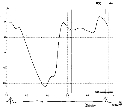
Looking at the strain rate and strain curves from one
singe heart cycle to the left, it is evident that while strain
(bottom) remains negative throughout the heart cycle, strain
rate (top) shifts between positive and negative. It can be
seen that the shifts from positive to negative (zero
crossings), in strain rate, corresponds to the shifts from
increase to decrease, or vice versa in strain (i.e. the peaks
and troughs in the curve). The peaks of the strain rate curve
on the other hand, corresponds to the change in the rate of
increase in the strain curve (of course), seen as the shifts
from concave to convex (or vice versa). The correspondences
are not perfect, as the strain rate is Eulerian,
while the strain is recalculated to Lagrangian,
as is the common convention. To the left are colour M-modes.
Strain rate (top) can identify the events by the
positive-negative shifts (blue-orange), while the peaks are
not discernible. But the colour M-mode discerns the
differences between event shifts in different depths. Strain
colour M-mode is not very useful in timing events.
Normal left
ventricular dimensions
Dimensions of the ventricle is closely related to the functional
measures. While the motion
indices of displacement and velocity are dimension unrelated,
strain
and strain rate are relative deformation measures,
and thus related to dimensions. Thus changes in dimensions will
relate to changes in strain and strain rate. The HUNT study, being
ta large study of normals has published normal values, related to
age and gender (386):
Conventional left ventricular cross sectional measures from
M-mode in the HUNT study by age and gender, raw and indexed for
BSA. SD in parentheses. From (386).
Age (years)
N
IVSd
(mm)
IVSd/BSA
(mm/m2)
LVIDd
(mm)
LVIDD/BSA
(mm/m2)
FS (%)
LVPWd
(mm)
LVPWd/BSA
(mm/m2)
RWT
RWT/BSA
Women
<40
207
7.5 (1.2)
4.2 (0.6)
49.3 (4.2)
27.5 (2.6)
36.6 (6.1)
7.7 (1.4)
4.3 (0.6)
0.31 (0.05)
0.17 (0.03)
40–60
336
8.1 (1.3)
4.5 (0.7)
48.8 (4.5)
27.3 (2.8)
36.5 (6.9)
8.3 (1.3)
4.6 (0.7)
0.33 (0.05
0.19 (0.03)
> 60
118
8.9 (1.4)
5.1 (0.8)
47.8 (4.8)
27.4 (3.1)
36.0 (9.1)
8.7 (1.4)
5.1 (0.8)
0.37 (0.07)
0.22 (0.04)
All
661
8.1 (1.4)
4.5 (0.8)
48.8 (4.5)
27.4 (2.8)
36.4 (7.1)
8.2 (1.4)
4.6 (0.8)
0.34 (0.06)
0.19 (0.04)
Men
<40
128
8.8 (1.2)
4.3 (0.6)
53.5 (4.9)
26.1 (2.6)
35.5 (6.9)
9.2 (1.3)
4.5 (0.7)
0.34 (0.06)
0.17 (0.03)
40–60
327
9.5 (1.4)
4.6 (0.7)
53.0 (5.5)
26.0 (3.0)
35.8 (7.4)
9.7 (1.4)
4.7 (0.7)
0.37 (0.07)
0.18 (0.03)
> 60
150
10.1 (1.6)
5.1 (0.9)
52.1 (6.4)
26.3 (2.9)
36.0 (8.0)
10.0 (1.3)
5.1 (0.7)
0.39 (0.07)
0.20 (0.04)
All
605
9.5* (1.5)
4.6† (0.8)
52.9* (5.6)
26.0† (2.9)
35.8 (7.5)
9.6* (1.4)
4.7† (0.7)
0.37 (0.07)
0.18 (0.04)
Total
1266
8.7‡ (1.6)
4.6 (0.8)
50.8‡ (5.4)
26.7 (2.9)
36.1 (7.3)
8.9 (1.6)
4.7 (0.7)
0.35 (0.07)
0.18 (0.04)
*p<0.001 compared to women. †p<0.01 compared to women.
‡Overall p<0.001 (ANOVA) for differences between age groups.
Wall thicknesses and LVIDD correlated with BSA (R from 0.41 - 0.48),
Thus, all values were consistently higher in men due to this. FS, of
course, did not correlate with BSA, and was thus gender
independent. Wall thicknesses increased with age (R=0.33),
while LVIDD and FS remained constant between age groups, in
accordance with other studies (387,
388,
389,
390).
Normal range is generally considered the interval between the 2.5
and 97.5 percentiles, ie. more or less mean ± 2SD.
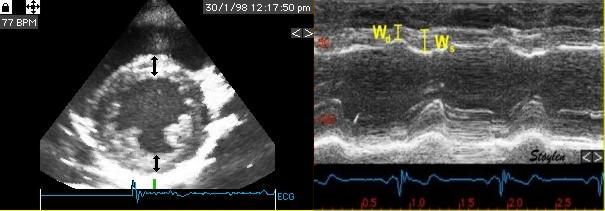
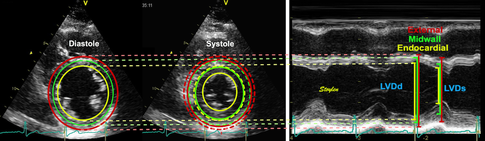
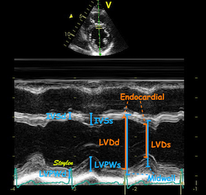
Wall thicknesses and chamber
diameters. RWT = (IVSd + LVPWd)/LVIDd, but there was no
difference if we used LVPWd x 2 / LVIDd. FS = (LVIDd -
LVIDs)/LVIDd. Left ventricular external diameter; LVEDd
= IVSd + LVIDd + LVPWd.
Left ventricular length. Wall
lengths were measured in a straight line (WL) in all six
walls from the apex to the mitral ring. This wil
underestimate true wall lengths (dotted, cirved lines),
but will be more reproducible, as the curvature may be
somewhat arbitrary. LVL was calculated as mean of all
four walls, thus overestmating true LVL (yellow line)
slightly, but again the arbitrary placement in the
middle of the ostium will result in lower
reproducibility, while taking the mean of six
measurements will increase it.
Relative wall thickness
Relative wall thickness is generally considered to be a body size
independent measure, as both wall thicknesses and LVIDD are body
size dependent, the RWT, supposedly, is normalised for heart size,
and hence, for body size. Interenstingly, in the HUNT study this was
not the case, although correlation with BSA was very modest
(R=0.18). This probably do not warrant normalising RWT for BSA. More
pronounced was correlation with age (R=0.34). The age dependency is
a logical consequence of the unchanged LVIDd and increasing wall
thickness, and has been shown also previously (391).
Relation of RWT and BSA. This shows
that RWT is not perfectly aligned with body size.
RWT and age. This shows a more
marked dependence of RWT and age, so age related normal
values is probably warranted.
Current guidelines recommend a cut off value of 0.42 between normal
and concentric geometry (146)
without taking age into consideration. In HUNT, however, the normal
upper limit is also closer to 0.52 over all.
The age relation is not taken into account either, as upper normal
limit is increases with age, from 0.41 to 0.54 in women and 0.44 -
0.54 in men, so age related values is warranted, unless one will
consider that all > 60 years have concentric geometry.
Left
ventricular length and external diameter:
Left ventricular length and external diameter is also important in
an evaluation of the total strain images. We measured these in the
HUNT study as well:
Left ventricular length and external diameter by age and gender
from the HUNT study, raw and indexed for BSA. From (386).
Age (years)
N
LVEDD (cm)
LVEDD/BSA (mm/m2)
LVL (cm)
LVL/BSA (cm/m2)
LVL/LVEDD
Women
<40
207
6.45 (0.48)
35.9 (2.7)
9.4 (1.6)
5.23 (1.00)
1.46 (0.26)
40–60
336
6.52 (0.52)
36.5 (3.2)
9.1 (1,7)
5.08 (0.95)
1.40 (0.27)
> 60
118
6.52 (0.52)
37.7 (3.5)
8.9 (1.3)
5.08 (0.79)
1.36 (0.23)
All
661
6.51 (0.51)
36.5 (3.2)
9.1 (1.6)
5.13 (0.93)
1.41 (0.27)
Men
<40
128
7.16 (0.53)
35.0 (2.9)
10.3 (1.7)
5.02 (0.88)
1.44 (0.25)
40–60
327
7.22 (0.58)
35.0 (3.2)
10.0 (1.8)
4.84 (0.89)
1.39 (0.26)
> 60
150
7.22 (0.68)
36.5 (3.1)
9.5 (1.8)
4.80 (0.97)
4.80 (0.97)
All
605
7.21 (0.59)
35.3 (3.1)
9.9 (1.4)
4.86 (0.91)
1.38 (0.27)
Total
1266
6.84 (0.65)
36.0 (3.2)
9.5 (1.8)
5.00 (0.93)
1.40 (0.27)
Left ventricular external diameter, is simply the sum of the wall
thickensses and LVIDd, so it is logical that this increased both
with BSA (R=0.60) and modestly with age (R=0.11, the unchanged LVIDd
being part of it, dilutes the effect of wall thickness) (386).
Left ventricular length, on the other hand, increased with BSA
(R=0.29), but decreased with age (R = -0.12).
Fundamental findings are summarised below:
Fundamental findings in the HUNT
study: With increasing BSA, both wall thickness,
internal diameter (and hence, external diameter) and
relative wall thickness increase, showing that neither
measure is independent of body size (or heart size). The
length / external diameter, however, remains body size
independent, being a true size independent measure.
Differences are exaggerated for illustration purposes.
With increasing age, both wall
thickness (and hence, external diameter) increase, while
internal diameter is age independent. Left ventricular
length decreases, and hence length / external diameter
decreases, and i a measure of age dependent LV
remodeling. This has implication for LV mass
calculation. Dimension changes are exggerated for
illustration puposes.
Ratio between
LV length and external diameter
The ratio L/D did not correlate with BSA, was near gender
independent (although the difference was significant due to the high
numbers), but declined somewhat more steeply with age (R = -0.17).
This has some important corollaries:
LV shape in healthy adults, is in itself a physiological
measure
Normalising cross sectional measures to LV length, corrects
better for heart size than normalising for BSA
The ratio L/D is a measure of age dependent remodeling in
healthy adults
LV mass calculations based on cross sectional (M.mode
measures), will over estimate LV mass increasingly with age, and
the assumption of age dependent mass increase with age may not
be valid.
The L/D ratio may be a new measure of LV hypertrophy.
Wall lengths per wall
Different walls has different lengths. In the HUNT study, the wall
lengths differed: Diastolic lengths of different walls (Mean and SD) measured in a
straight line from apex to mitral ring, by age and gender. Only
over all values are published in (386):
Age (Years)
Septum
Lateral
Mean of two; septal and lateral
Anterior
Inferior
Mean of four; Septal, lateral, anterior, Inferior
Anteroseptal
Inferolateral
Mean of all six
Women
<40
9.0 (1.6)
9.4 (1.6)
9.2 (1.6)
9.4 (1.7)
9.3 (1.6)
9.2 (1.6)
9.2 (1.9)
9.8 (1.6)
9.4 (1.6)
40-60
8.8 (1.6)
9.1 (1.7)
9.0 (1.6)
9.2 (1.7)
9.1 (1.7)
9.0 (1.6)
8.9 (1.9)
9.6 (2.1)
9.1 (1.7)
>60
8.5 (1.3)
9.0 (1.4)
8.7 (1.3)
8.9 (1.4)
8.8 (1.3)
8.8 (1.3)
8.5 (1.6)
9.4 (1.7)
8.9 (1.3)
All
8.8 (1.5)
9.2 (1.6)
9.0 (1.6)
9.2 (1.6)
9.1 (1.6)
9.1 (1.6)
8.9 (1.9)
9.6 (2.0)
9.1 (1.6)
Men
<40
9.9 (1.7)
10.3 (1.8)
10.1 (1.7)
10.2 (1.8)
10.3 (1.8)
10.2 (1.7)
10.1 (1.8)
10.8 (1.9)
10.3 (1.7)
40-60
9.7 (1.7)
10.2 (1.8)
9.9 (1.7)
10.0 (1.8)
10.1 (1.8)
10.0 (1.7)
9.5 (1.9)
10.6 (2.2)
10.0 (1.8)
>60
9.1 (1.8)
9.7 (1.9)
9.4 (1.9)
9.4 (2.1)
9.5 (2.1)
9.4 (1.9)
9.1 (1.9)
10.2 (2.1)
9.5 (1.9)
All
9.6 (1.8)
10.1 (1.8)
9.8 (1.8)
9.9 (1.9)
10.0 (1.9)
9.9 (1.8)
9.5 (1.9)
10.5 (2.1)
9.9 (1.8)
Total
9.2 (1.7)
9.6 (1.8)
9.4 (1.7)
9.5 (1.8)
9.5 (1.8)
9.5 (1.7)
9.2 (1.9)
10.1 (2.1)
9.5 (1.8)
All lengths in cm.
The lateral and inferolateral walls were significantly longer than
all other walls (including each other). The septum and anteroseptal
walls were significantly shorter than all other walls. Means of two,
four and six walls were all significantly different from each other,
but the differences were negligible, considering that the limit for
measurement accuracy is 1 mm.
Left ventricular volumes
Applying the linear measures to an elliptical model of the left
ventrcle, allowed the estimation of LV volumes (471).
Ellipsoid model of the left ventricle. All
basic measures are linear, and the ellipsoid model assumes
symmetrical wall thickness, declining to half in the apex,
mitral annular diameter constant; equal to ventricular end systolic
diameter, as LV diameter decreased by 12.8% is systole while
the fibrous mitral annulus may be assumed to be more constant.
The ellipsoid model has some limitations. Being symmetric, it do
not conform totally to the shape of the LV, which is assymmetric,
as in other model studies.
An indication of this was that while all linear measurements were
near normally distributed, there was a greater skewness in the
calculated volunes:
Comparing skewnesses of the distributions of
the linear measures (which is small), with the calculated
volumes (which is significantly (greater), seems to indicate a
systematic error in the volume data from the model.
Despite this, it was interesting findings.
LV volume and age
As we have already shown, left ventricular wall thickness increased
with age, LV diameter was unchanged, while LV wall length decreased
(386).
However, LV volume increased by age (471).
But the HUNT 3 population despite exclusion of patients with history
or treatment for hypertension, had an increasing mean SBP and DBP
with increasing age, due to an increasing number with BP above
hypertensive levels:
A: Mean BP showing an age related increase,
above 60 about half is in the hypertensive level >140/90.
B: LV volume in the different BP groups (results were not
different if 140/90 was used). There is significant higher
volumes in the >130/80 group, but in neither group was
there any significant increase with increasing age.
There was a weak, but significant correlation of LV volume with age
(R=0.14, p<0.001), but neither in linear regression nor partial
coorrelation was there any significant increase with age, indicating
that the age effect is mainly an BP effect.
Geometry of
myocardial strain
Still preaching my
personal litany: Strain is geometry.
(Cormorant, Galway, Ireland).
Normal strains,
longitudinal, transmural, circumferential.
Myocardial directions -
normal strains
As described in "basic
concepts"section, the strain tensor has three normal strains (11)
in the x, y and z directions in a Cartesian coordinate system. Also,
in an incompressible object, meaning that deformation doesn't affect
volume, the three strains have to balance by the incompressibility
equation: .
Strain in the heart also has three main components, but the
directions are customary related to the most common coordinate
system used in the heart: Longitudinal, circumferential and
transmural. (The term "radial" is often used to describe transmural
direction, but as this in ultrasound terms may also mean "in the
direction of the ultrasound beam" in the ultrasound
specific
coordinate system, "radial" strain is ambiguous and should be
avoided. Transmural strain is unambiguous).
The two coordinate
systems are equivalent, but the cardiac system are more practical
for a hollow body.
Left, the xyz coordinate systems relating to the deformation
of a cube. Right the LTC coordinates of the LV myocardium,
which in principle is equivalent as shown here.
In both cases there is ONE deformation of a three
dimensional object, which deforms in three dimensions, and the
three normal strains are the coordinates of this deformation.
As wen would not talk about the xyz deformations of a cube as
three independent functions, it is not appropriate to talk
about three independent myocardial functions. Below are the
strain tensors for the xyz and ltc deformations. In both
cases, there is one tensor with three normal components.
From this, it is evident
that the three strain components are components of ONE tensor, and
are the coordinates of ONE deformation of a three dimensional object
in three dimensions. It makes very little sense to consider this
equivalent to three independent functions in three directions. (One
would not consider the xyz strains of a deforming cube as three
independent functions, so why do that in the cardiac coordinate
system?
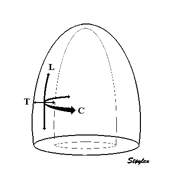
Strain
in three dimensions. In the heart, the usual directions
are longitudinal, transmural and circumferential as
shown to the left. In systole, there is longitudinal
shortening, transmural thickening and circumferential
shortening. (This is an orthogonal coordinate system,
but the directions of the axes are tangential to the
myocardium, and thus changes from point to point.)
This long axis video shows
how the apex is stationary, while the base moves toward
the apex in systole, away from the apex in diastole.
This means the ventricle shows strain between apex and
base. Longitudinal strain will be negative (shortening)
during systole and positive (lengthening) during
diastole (if calculated from end systole).
This short axis video shows
both transmural and circumferential strain. Systolic
transmural strain equals wall thickening. Systolic
circumferential strain is the systolic shortening of any
of the countours; outer, midwall or endocardial, The
change in outer contour is least, while the endocardial
contour shortens most, thus, there is a gradient of
circumferential strain across the wall. This is
explained below.
The strain components are simply coordinates of the three
dimensional deformation of the myocardium, and has nothing to do
with material properties of the myocardium, such as anisotropy or
fibre directions in a direct sense. Of course, the total deformation
is a function of fibre shortening, and ultimately, among other
things fibre architecture, but also of load and valve function. And
it is of note, that while systolic deformation deformation continues
to end ejection, myocardial relaxation starts at peak pressure.
Thus, systolic deformation in the heart occurs in all three
dimensions simultaneously.
It is evident that
Lagrangian strain is well suited to describe systolic
deformation. Diastolic thinning or elongation, however, is not
so well described by Lagrangian strain as Lo
is defined in end diastole.
Circumferential
strain
= relative shortening of one of the
circumferences (external, midwall or endocardial).
The concepts transmural displacement and transmural velocity are in
reality meaningless in a physiological sense. The displacement and
velocity in the transmural direction is dependent on where across
the wall it is measured, i.e. the transmural depth of the ROI
placement. Different data sets from tissue Doppler in the transmural
direction is thus not comparable, and the measurements have little
clinical value. Some applications like 2D
strain will give the segmental average value for transmural
velocity and displacement. They may have a clinical meaning, in that they may separate normal
from reduced function, but the use of clinical measurements that are
physiologically unsound, is doubtful.
Since strains are simple deformation measures, linear strains can be
measured by end systolic and end diastolic measures in three
dimensions:
Linear strains in three dimensions.
Longitudinal shortening. Longitudinal strain can be measured
by systolic and diastolic left ventricle (LV) lengths (A) or
by Annular motion (B) divided by wall lengths (A). Transmural
strain to be a truly segmental measure (C), the quantitative
equivalent of wall motion score. The circumferential strains
can be seen to be related to outer circumferential shortening
as well as wall thickening, and endocardial circumference can
be seen to move most, external most. As circumferences
can be calculated from diameters, circumferential strains can
be calculated from fractional shortening. Midwall and external
circumferential strains were calculated from endocardial
diameters and wall thicknesses.
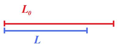
Longitudinal strain
Longitudinal strain, being relative longitudinal systolic
shortening, is, from the Lagrangian
definition of strain, it follows that longitudinal strain is:
. It
follows from the formula, that as there is systolic shortening,
systolic longitudinal strain is negative (systolic length smaller
than diastolic).
Longitudinal shortening of the
left ventricle. Lagrangian strain is the relative
shortening normalised for the end diastolic length.
LV shortening can be
measured by M-mode as the MAPSE, the
relative shortening is the normalised MAPSE = MAPSE /
L0.
An example:
Systolic strain is
normalised MAPSE. The normalised MAPSE for this ventricle
with an end diastolic length of 9.8 cm and an MAPSE of 17 mm
is 15 / 92 = 17.3. This corresponds to a longitudinal
strain of -17.3% in this example.
In the HUNT study, MAPSE as mean of 4 walls was 1.58 cm (417, 456).
Mid ventricular end diastolic length was 9.24 (), and
longitudinal strain by this method was -17.1%. However, this is not ambiguous. In
the HUNT study, we measured the distance from the apex to the
mitral points, in lieu of wall length (WL). This ensured
better reproducibility, the mitral points being more defined
that the mid LV point.
Over all ventricular strain should
be as illustrated above. Basically, Global LV strain (GLS)
strain is LV
shortening normalised for LV length, GLS = MAPSE / LVL
(normalized
displacement), and for Lagrangian strain, this the
denominator is end - diastolic length (L0).
Linear strain
Strain by WL is
numerically smaller than by LV length, as the
denominator is bigger (WL>L).
But following the
curvature of the wall, would result on an even
longer WL, a higher denominator and a numerically
even smaller strain.
In the HUNT study, Mean diastolic WL was 9.47 cm, and mean
strain by MAPSE/WL (calculated per subject an wall an then
averaged, was -16/3%, as WL is longer than LV length, as
evident from the figure above. We did not do the curved wall
exercise at that time, as the data quality was less, and
automated edge detection was not so good. It might be done
now, in later databases with newer generation scanners, if
deemed worth while.
As shown above, wall length can be
measured in different ways, which has consequences for strain
measurement. The lowest
denominator as illustrated above, is the mid chamber line (L0), giving
the highest numerical GLS value. Normalising for wall
lengths instead, will give a higher denominator, and thus a
lower numerical GLS
value. One approximation to wall lengths is to use the
straight line from apex to the mitral points. This will give
a high reproducibility by using clear anatomical landmarks,
and the straigh line is reproducible. In addition, there
will be little angle difference between the M-mode line and
the wall line, in effect eliminating the systematic angle
error. This is the linear strain method (417,
444)
described here,
resulting in a mean strain of 16.3 (2.4)%.
This is also illustrated by the examples below. .
For any given MAPSE, the global strain will
be determined by the choice of denominator. In this case,
mean MAPSE is 1.7 cm. End diastolic length will be the
denominator in the strain equation. Using the mid
ventricular line (blue), gives the smallest denominator
and thus the highest global strain value of 17.3% in this
example. Using wall length, will result in a higher
denominator, resulting in lower GLS value, the straight
line approximation (green) gives an intermediate
denominator and a GLS value in this example of 16.3%,
while the curved lines (red) following the walls gives the
highest denominator, and thus the lowest GLS value, in
this example 14%.
Another example:
Illustration on how the choice of reference length
will affect the strain value. The curved lines, representing
the longest wall measurements, will give the lowest GLS
value, the straight lines will be in between, while the mean
ventricular length will be the shortest, and thus give the
highest strain value.
Choosing instead the curved wall line, will give a truer
length, at the cost of higher variability, but the length will
be systematically higher, resulting a higher denominator and
lower value of GLS as shown above. In this case, there is a
lagrangian strain using only the end diastolic length, as
opposed to speckle tracking as shown below.
Speckle tracking strain
Speckle tracking strain in general not only have
curved ROIs, but also tracks crosswise motion of the speckles,
which is due to wall thickening. As the wall thickens, this means
that speckles move inwards in the cavity. Let us consider a
hypothetical example where there is wall thickening without wall
shortening. (This would mean volume expansion, but illustrates
still the effect of wall thickening.):
Hypothetical wall thickening without wall
shortening. As the wall thickens, both the midwall (red
unbroken) and the endoicardial (blue unbroken)line moves
inwards. This is true for both the curved line (depending on
the curvature) and the straight lines (depending on the
cosine of the angle change), the inward motion shortens the
lines.
Thus wall thickening results in inward motion, even without wall
shortening, and thus the tracking itself will introduce an element
of strain that is not true wall shortening. The real story, of
course, is that there is simultaneous wall shortening and
thickening, and the thickening
is mainly a function of shortening, due to conservation of
myocardial volume.
Simultaneous wall shortening and thickening. As
the wall shortens, it has to thicken, due to conservation of
the myocardial volume. As illustrated above, the mid and
endocardial lines shorten not only due to wall shortening,
there is a shortening due to the inward movement as well,
which again is caused by wall thickening. And as wall
thickening is due to wall shortening, this means that the
shortening is speckle tracking strain is over estimating the
true wall shortening.
This means that speckle tracking strain, tracking both longitudinal
and inward motion, is really incorporating the effect of wall
shortening twice, and thus over estimates the true shortening
systematically. The endocardial line will move more inwards (being
displaced by the thickening of the whole wall), while the midwall
line will be displaced only by the thickening of the outer half of
the wall, just as for circumferential
strain(255, 456).
Global strain is a mean value of the strain within the ROI. Using an
ROI with a certain thickness, the mid ROI line can be considered a
reasonable proxy for mean global values.
This may be a reason for why speckle tracking GLS (423,427,447-449) is higher than what we found with segmental strain (153),
and also what we and other have found with linear strain (417,444), and in my opinion
actually has a systematic over estimation of the true wall
shortening.
Thus, speckle tracking strain is expected to show higher
absolute values for GLS than linear strain, or non tracking
methods. A large meta analysis gave mean normal values of 19.7%
(427),
but the study was unable to show age or gender variability due
to large inter study heterogeneity. The NORRE study (457)
found in a single center speckle tracking study a GLS of mean
22.5 % (SD2.7). This is as expected.
Segmental strain
Measuring strain per segment will give the global strain as
the mean of all segments. In the HUNT study, we measured segmental
strain by the longitudinal segmental method tracking kernels at
the segment borders by tissue Doppler in the longitudinal
direction, and speckle tracking in the transverse direction, as
described here.
Segmental strain by tracking kernels at the
segmental borders, calculating strain as relative segment
length shortening, and GLS as mean of all segments.
This method was used in the first
publication from the HUNT study (153).
In this study, the mean GLS was 16.7 (2.4)%, so there is a fair
correspondence between linear strain and this segmental method.
However, all inward tracking will be affected by wall
thickening, adding an element of shortening that is a systematic
error as shown below. I would expect this to be subject to the
same error by inward tracking as ST, but as this application
used TDI data with a low underlying B-mode FR and lateral
resolution, the lateral tracking may have been so poor, the
technical shortcoming offset the systematic error.
As with all other strains, speckle tracking strains rest on
assumptions: , width of the ROI, In addition, the black box ST
applications all have complex algorithms with
different choices for
-Assumptions of LV shape and ROI width
-Mid/mean vs
endocardial
-Number, size and stability of speckles
-Decorrelation detection and correction
-Spline smoothing along the ROI and weighting of the AV -plane
motion
-Etc.
However, there are additional assumptions that will
differ between vendors of speckle tracking programs. Using mean
strain over the ROI will result in a value close to the mid ROI
line. Some vendors, however, trace the endocardial line, which
will result in higher absolute values. The thickness of the ROI is
often assumed to be constant, while the wall is thinner in the
apex. As the apex is the most curved part, a ROI in the apex that
is thicker than the wall, will result in a higher absolute GLS.
The curvature in the apex may also vary, even in the same
software, as shown here.
Curvature dependency of
strain in 2D strain by speckle tracking.The two images are processed from
the same loop, to the right, care was taken to straighten out
the ROI before processing, while the left was using the
default ROI. In both analyses the application accepted all
segments. It can be seen that the apical strain values are far
higher in the right than in the left image (27 and 21% vs 19
and 17%). However, the curvature of the ROI even affects
theglobal
strain, as also discussed above in thebasic
section.
Finally smoothing,
software algorithms, such as choice of kernel sizes, selection and
weighting of acoustic markers, stability of speckles, and drift
compensation during heart cycle are all assumptions that are
guarded as industrial secrets.
Thus, it is not surprising that there are inter
vendor differences, even in speckle tracking derived strain.
Inter
vendor differences in speckle tracking
As speckle tracking have been
attempted to be a solution to the shortcomings of tissue Doppler,
and as this can be done in ordinary B-mode. most vendors have in
time come up with speckle tracking applications in their analysis
software. Also, vendor independent software, using the DICOM
standard, are available.
This has been an interesting
development, as the later studies have shown a fair amount of
variability between strain measurements by different vendors (373 - 382). Normal values are not
sufficiently harmonised that measures are interchangeable. For
longitudinal 2D strain, biases of 1% absolute (373- but here both
methods had a much larger bias against MR tagging), to 5% (375).
and with correlations between
measurements in same-day measures in the same patients vendor
specific software as low as 0.35 (374)
to 0.23 (377),
but with no or less differences between different acquisitions
when analysed in the same software (374),
suggesting that the differences in software is the main source of
variability between systems. However,even different versions of the same
software has been shown to result in different measurement values
(377).In general, variability have been
found to be between 2 and 5% between software (378).
It has been suggested that reproducibility is better than for EF
measurements, but taking into account that EF by biplane tracings
isthepoorest reproducible
parameter, this argument does not impress much.
Reproducibility within the frame
of one software vendor, is much better, not surprising as
discussed years ago in the paragraphabove, thesmoothingwill always yield
good repeatability (in fact, if you smooth the curves to zero,
repeatability will be 100%), but still it has been found to be
unacceptably high in newer studies, even within the frame of one
software (377).
Although some researchers have
found a fair correspondence between global strain measurements, (376),
reproducibility of regional strain is much poorer.
It's important to realise that different applications may measure
strain in different ways as indicated above, and as shown
elsewhere. 2D
strain measures along the curved line following the wall, the
M-mode
method as well as Tissue Doppler will measure along the
ultrasound beam, being a straight line, while segmental
strain will measure along a straight line in each segment,
thus being somewhat in between, as shown by this
figure. Also, there is a slight difference between longitudinal
stain measured in the midwall compared to endocardial measurement,
due to the inward shift being more pronounced in the endocardium as
discussed below,
as well as due to the fact that the midwall line is slightly longer
than the endocardial, thus giving a larger denominator in the strain
expression.
Thus, global longitudinal strain will vary with processing software
(vendor).
Now, the EACVI/EAE task force has
recommended that for speckle tracking, the denominator should be the
line following the myocardial wall, whether it is is the endocardial
or midwall, and also that the level should always be reported by the
software (287).
However, this is for the speckle tracking applications
only, as it is not feasible (or indeed possible) for
tissue Doppler, nor for normalised
MAPSE. And some of the comments are not valid for segmental
strain by speckle
tracking either. (The recommendations explicitly are for
2D speckle tracking only).
Secondly, some ambiguity remains, as applications where the
ROI has the same width in the base and apex, despite the
differences in thickness of the myocardium. In this case, at
least one side of the ROI will not follow the wall, and the mid
line of the ROI will not follow the midline of the wall (or, if
the ROI are suited to the midline, the endocardial side of the
ROI will not follow the endocardium). If so, the results may
vary as shown in the figure below:
There is no gold
standard for longitudinal strain
As there is no universal algorithm forglobal strain, of course the concept of global strain as a universal
measure of ventricular function has no exact meaning. It is only
a theoretical concept. This means there is no reference standard, they are
method dependent. This means that strain values cannot be
validated, and different methods cannot be compared in terms of
validity, and finally, normal values do only have validity
within the method used.
There is no universal definition, and
thus no "ground truth" at all for GLS. Methods cannot be
validated, and GLS has to be considered only within the method
used.
Is
there layer specific longitudinal strain, and can we measure
it?
It is discussed below
that there is a gradient of transmural and circumferential strain,
but due to pure geometry.
Normal transmural
gradient of longitudinal strain.
A transmural gradient of longitudinal strain has likewise been
published (371).
Looking
at the speckle tracking of longitudinal strain as discussed above,
there will be a component of shortening that is due to the tracking
of inward motion caused by wall thickening, just as in
circumferential strain. And this effect increases from the
epicardium to the endocardium, just as for circumferential
strain, as the midwall line is pushed inwards by the outer
half of the wall thickening, while the endocardial line is pushed
inwards by the whole wall thickening.
Hypothetical wall thickening without wall
shortening. As the wall thickens, both the midwall (red
unbroken) and the endoicardial (blue unbroken)line moves
inwards. This is true for both the curved line (depending on
the curvature) and the straight lines (depending on the cosine
of the angle change), the inward motion shortens the
lines.
Thus the gradient of layer strains can be explained solely by the
tracking effect of wall thickening. If there had been an additional
increase in endocardial longitudinal strain, this would have
resulted in systolic torsion of the mitral ring, which, being part
of the larger fibrous AV-plane, is counter intuitive. To say nothing
of what that would have caused for the rest of the AV-plane and the
RV!
Proposed geometry if there should have been more
absolute shortening in the inner layer, this would mean a
torsion of the mitral plane in systole as illustrated here by
the rise of the inner part, but this is inconceivable, the
mitral plane is part of the larger fibrous annular plane.
This again, is solely a function of the geometry of myocardial
thickening, and the way strain is measured, and the fact that the
endocardial parts have to thicken more, due to the decreasing space
analoguous
with the circumferential strain, if motion due to wall
thickening is followed.
Transmural strain
Transmural strain is simply relative wall thickening. There is no
such thing as "transmural myocardial function", as there are no
transmural fibres. Wall thickening is solely due to
incompressibility; as the wall shortens, in the longitudinal,
and eventually also in the circumferential direction, it must
thicken in the transverse direction to conserve myocardial volume.
It is very evident that longitudinal and transmural strain are not
independent.
Longitudinal shortening can easily be demonstrated in apical echo
images as shown above,
as well as measured as shown below. Transmural thickening is
equivalent to wall thickening, but from the images below, it is
evident that the wall has to thicken as it shortens in order to
conserve volume (NOT MASS!!!).
Ventricular
strain. Diastolic and systolic images of the heart.
Systolic shortening of the left ventricle relative to
diastolic length, is the systolic strain of the
ventricle. From the Lagrangian definition of
linear strain; , it follows that systolic
longitudinal strain is:
However,
it is also evident from this image, that as the wall
shortens, it also thickens, to conserve the volume.
Heart muscle is generally assumed to be incompressible.
Schematic diagram of the left
ventricle, showing the relation between shortening and
wall thickening (exaggerated for illustration purposes),
with a model of unchanging outer contour in an
incompressible myocardium.
Wall thickening, illustrated from
the loop shown to the left. The outer (red) and
endocardial (yellow) contours and wall thicknesses are
shown in the diastolic image to the left, and
transferred to the systolic image on the right, shown as
dotted lines of the same colour. The systolic contours
are shown as solid lines. The systolic wall thickness is
then (more or less) the dotted plus the solid blue
lines, and the wall thickening the solid blue lines.
Transmural strain is a purely segmental measure. Global transmural
strain either has to be measured in all 16 segments, (three
parasternal short axis planes), or inferred from assumptions of
symmetry.
What is very evident here, is that transmural strain in fact is a
quantitative equivalent to the semi quantitative wall
motion score.
Speckle tracking, however, is not necessary for transmural
strain. Wall thickening can be measured by simple caliper
measurements of wall thickness in systole and diastole. It is still
segmental, but can be generalised from fewer measurements under
assumptions of symmetry, as has been done from M-mode. The
transmural strain can be measured in M-mode from systolic and
diastolic wall thickness, which will give wall thickening in only
two segments, but may be taken as representative as the mean wall
thickening in this plane where there is no segmental dysfunction.
However, in this case, generalizing from M-mode measurements, the
sepal and inferiolateral wall should be averaged, as septal
thickening is less than inferiolateral wall thickening (392):
Transmural
strain by M-mode. The M-mode measurement is more accurate
than 2D measurements, but are only feasible in the septum
and inferolateral (posterior) wall. Thus, the transmural
strain can only be extrapolated in symmetric ventricles. Strain by tissue
Doppler is also only feasible in the two walls
perpendicular to the ultrasound beam as indicated by the
arrows.
If using M-mode, however, the
average of septal and inferolateral wall should be used,
as septal thickening is less than inferiolateral wall
thickening.
Thus:
There is no such thing as transmural function. Transmural
strain is thus in itself not a function measure. This is hardly
surprising, as there are no transmurally directed fibres. Wall
thickening reflects the thickening of the individual muscle fibers
inn all directions as they shorten.
Depending on how much or little change there is in outer contour,
the transmural strain will mainly be a function of longitudinal
shortening. Wall thickness and cavity diameter are also geometric
determinants of wall thickening. However, in any given ventricle
with a given cavity diameter and end diastolic wall thickness, the
transmural (radial) strain is mainly a function of longitudinal
strain, not an independent measure.
However, transmural strain will be very much influenced by
processing, especially ROI size (276),
as discussed here.
Radial strain values from the two
different ROI's to the left, showing again a huge effect of
ROI width on transmural strain values.
There will be a gradient of transmural strain from the epi- to the
endocardium. As the wall thickens, the endocardial layers expand in
a space with a smaller circumference, and thus they have to thicken
more for the same volume increase. But this is due to geometry, not
to any gradient in layer function.
Illustration of the
gradient of wall thickening. A:
diastole. B: hypothetical thickening of the outer layer (red).
This pushes the inner layer inwards, where the circumference
is smaller, thus, there is less room. Thus, this displacement
itself causes the inner layer to thicken. This comes in
addition to the intricsic thickening of the inner layer by
shortening, and thus, the inner layer thickens more than the
outer, simply becuse of less room. Even without presupposing circumferential fibre
shortening, there is thus inward shift
of midwall and endocardial contours as the wall thickens. And as the midwall contour is only
pushed inwards by half the wall thickening, there is a
gradient of circumferential shortening, and thus the two are
different.
As stated above, transmural strain is a measure of deformation, not
of function. It is simply a component of the strain tensor, or a
coordinate of the total deformation.
If there is a component of circumferential fibre shortening, this
must mean that there will be a decrease in outer diameter, which
then also contributes to wall thickening.
Wall thickening as a function of longitudinal shortening.
Calculated from a hypothetical, symmetric, half ellipsoid model
with a diastolic mid wall thickness of 0.9 mm (decreasing
towards apex), an outer diastolic diameter of 60 mm, a diastolic
length of 95 mm. Wall thickening is calculated from longitudinal
shortening and conservation of wall volume, given different
degrees of outer contour change (outer circumferential strain or
shortening). Longitudinal strain given in negative
values; i.e. wall thickening increases as THE VALUE of
longitudinal strain increases. As seen here, if there is no
outer diameter reduction, the wall thickening is solely a
function of wall shortening.
Circumferential strain
Circumferential strain means shortening of a circumference in the
ventricle.
As transmural strain,
circumferential strain must be measured in short axis
planes.
External circumference is shown in
red, midwall circumference in blue, and endocardial
circumference in orange. The circumferences from the
diastolic left frame are shown as dotted lines of the
same colour in the systolic frame to the right, to
compare with the systolic contours in unbroken lines.
The inward motion is evident, and there is a gradient
from outer to inner contour.
When considering circumferential shortening, three points is
important:
Circumferential shortening is to a large degree due to the
inward shift of the circumferences as the wall thickens. thus:
Even without any change in outer contour, the endocardium will
shift inwards as the wall thickens, and there will be both
endocardial and midwall circumferential shortening
There would have been circumferential shortening even if there
had been no circumferential fibres, as the wall thickening due
to shortening would give this inward shift, as long as the
pericardium would counteract the ecpansion by the pressure
generated by the longitudinal shortening.
This means that there is fairly little relation between
circumferential fibre action and circumferential strain, except for
the outer contour. The main function of the circumferential vectors
seems to be balancing of the intracavitary pressure, but this is
isometric, and do not necessarily cause shortening.
The circumferential strain in a normal ventricle is the shortening
of a circumference due to the inward shift caused by the wall
thickening. Even if there had been no circumferential fibres,
there would have been wall thickening and thus circumferential
strain (as long as the pericardium would hold against
the pressure generated by longitudinal shortening).
Circumferential strain
is an ambiguous term.
The circumferential strain has no meaning except as a shortening of
a defined circumference. As circumferential strain is mostly due to
the inward shift of the various circumferences, all but the outer
circumferential strain are partly a function of wall thickening.
This means
And this is dependent on which circumference, as circumferential
shortening increases from the epicardium to the endocardium.
Thus, there is a gradient of circumferential strain from the outer
to the inner contour, (due to geometry NOT to layer specific
function).
Different software today use different definitions, some measuring
endocardial, others midwall circumferential shortening. Thus, there
is no standard circumferential strain, it is is method dependent.
Normal
transmural and circumferential strain gradients
There is a normal gradient of strain from outer to inner contour.
This has been confirmed emprically (255
,456,
457).
In the HUNT study (456)
the circumferential strains are:
Endo-card εC
Midwall εC
External εC
-36.1 (7.3)
-22.7 (4.9)
-12.8 (4.0)
This, however, has got nothing to do with differences in fibre
function, but is simply due to geometric factors,and is
already discussed in the paragraph on circumferential
strain.
transmural gradient of strain. The thickening of the
outer layer displaces the inner layer inwards. This alobe will
cause the inner layer to thicken, due to being pushed into a
region where the circumference is smaller, and thus thickening
has to compensate in order to preserve layer volume. The
thickening of the inner layer due to shortening, comes in
addition to this, and thus the inner layer has to thicken more
than the outer layer. Thus, there is a gradient of ttransmural
strain across the wall, increasing towards the endocardium.
But this also is the case for circumferential strain. The mid
circumference of the outer layer moves inwards (and hence,
shortens) according to the thickening of the outer layer. The
midwall line of the inner layer moves inwards (and hence,
shortens) both due to the inward shift of the inner alyer, and
due to the increased thickening of the inner layer. Thus there
is a gradient of circumferential strain increasing towards the
endocardium as well.
The gradients of transmural and circumferential strains are thus a
function of geometry alone in the normal ventricle, simply as the
myocardium nearest the inner wall is pushed more inwards, and thus
have to both thicken and shorten more due to reduction in available
space.
Midwall and endocardial strain as
functions of wall thickening, for 0%, 5% and 10% outer
diameter reduction.
As wall thickening also is a
function of longitudinal strain, midwall and endocardial
strain as functions of longitudinal strain, for 0%, 5%
and 10% outer diameter reduction.
Calculated from a hypothetical,
symmetric half ellipsoid model with a diastolic mid wall
thickness of 0.9 mm (decreasing towards apex), an outer
diastolic diameter of 60 mm, a diastolic length of 95 mm. Wall
thickening is calculated from longitudinal shortening and
conservation of wall volume, given different degrees of outer
contour change (outer circumferential strain or shortening). Longitudinal
and circumferential strains are given in negative values; i.e.
wall thickening increases as THE VALUE of longitudinal strain
increases.
Illustration of the circumferential shortening from
diameter measurement, and how these can be derived from
M-mode.
The circumferential fibre shortening contribute to circumferential
strain, depending on how much reduction there is in outer diameter.
This will increase not only the shortening of the midwall and
endocardial surfaces, but also the gradient of shortening from outer
to inner surface. If the outer circumference shortens, there is less
room for the myocardium which has no alternative than expanding
inwards.
But again: If transmural strain is mainly a function of longitudinal
shortening, and circumferential shortening mainly a function of
transmural thickening, this means the three are inter related:
Thus, transmural and circumferential
strain can be summed as this:
Relations between
circumferential shortening, wall thickening and the transmural
strain gradient. There is a modest outer circumferential
shortening, (I.e. a modest reduction in circumferential diameter
and thus circumference. Longitudinal shortening leads to wall
thickening, which then is inward expansion of wall thickness,
and inward displacement of the other circumferences. The outer
layer (light red) is pushed inwards by the outer circumferential
shortening, but there is also a net thickening (bold, red
arrow), due to both the inward displacement, but mainly
longitudinal shortening. This wall thickening is an inward
expansion, displacing the midwall circumference (Dotted red
circle) inward, and thus, midwall diameter and circumference
shortens too. The inward thickening of the outer layer, leaves
less room for the inner layer (light blue), which then has to
thicken even more (net thickening; bold blue arrow), both due to
inward displacement, as well as due to the intrinsic thickening
(caused by shortening). Thus it has to thicken more, and the
endocardial circumference (dotted blue circle) is displaced more
inward, leading to more reduction in endocardial diameter and
circumference.
Actually, the fact that the inner layer thickens into a much less
space, means it has tho thicken more. But this also means that the
midwall circumference moves inward also in relation to the tissue
itself, and does not relate to then mid line of the tissue.
In order to talk about circumferential strain, first, the question
has to be answered: Which circumference? (external, midwall or
endocardial)
Circumferential
strain is a function of diameter reduction.
As the circumference is simply a function
of the diameter (C = * D), circumferential strain can be computed
directly from the diameter fractional shortening (i.e. midwall
or endocardial, respectively):
Thus, circumferential strain equals
fractional shortening!
(I.e. either endocardial or midwall)
As circumferential strain equals the negative value of fractional
shortening, it can be generalised from fewer measurements from
assumptions of symmetry, as has been done from M-mode. If the cross
section of the LV is assumed circular, the CS equals - FS.
Angulation of the M-mode line wil not matter, as this is the
relative shortening, which will remain constant.
Speckle tracking in short axis
image. The thickness follows the wall thickening, and
the mid line in the ROI shows midwall circumferential
shortening.
Midwall (blue) and endocardial
(orange) circumferential strain is equalt o the negative
value of fractional shortening, and thus, the mean
circumferential shortening of the short axis plane can
be measured from M-mode.
M-mode as well as short axis cross sections, may sometimes show
greater inward motion of the outer contour, due to the out of plane
motion of the base of the heart.
As can be seen, the base of the
heart moves through the M-mode line during the heart
cycle.
This means that measurements in
fact are taken from different part of the ventricle in
end diastolie and end systole. It seems to indicate that
systolic measurements are done in a part of the
ventricle withsmaller diameter, thus over
estimating inward motion of the outer contour.
Circumferential strain by
speckle tracking
The advance of speckle
tracking have enabled analysis of deformation in all
directions, although with severe
limitations inherent
in
ultrasound itself as well as due to the
specific applications for analysis. Speckle
tracking also gives the possibility of measuring smaller regions of
the myocardium. This may be subject to severe restrictions, however.
Also, measurements are related to geometry, which do not necessarily
relate to differences in fibre function.
Circumferential strain again is also available by speckle tracking
in short axis images:
Short axis cine loop
Speckle tracking in the same cine
loop
Resulting peak circumferential
strain strain values and strain curves from the
tracking. There is abnormal swtrain curves in the
inferior segments due to imperfect lateral tracking in
the remote region (reduced lateral resolution with
depth) as discussed int the pitfalls
section.
The advantage of speckle tracking is that no assumptions of symmetry
are necessary, so segmental differences can be assessed (although spline
smoothing is an issue also here).
T&he disadvantage of speckle tracking is that tracking is in the
lateral direction in the anterior and infrior walls, and resolution
(and thus tracking ability) is less in the lateral direction.
Especially the inferior wall, as lateral resolution decreases with
depth in a sector image.
This means that the measure of circumferential strain is
either segmental, measuring strain in separate segments,
or regional, the average circumferential strain in a short
axis plane is representative for that plane only,
and that the FS of that plane as measured by M-mode, is equal
to the average circumferential strain in the same plane.
The linear
strains, based on simple measurements as shown below. in three
dimensions in the HUNT3 study are given here, from (456).
Linear strains in three
dimensions. Longitudinal shortening. Longitudinal strain can
be measured by systolic and diastolic left ventricle (LV)
lengths (A) or by Annular motion (B) divided by wall lengths
(A). Transmural strain to be a truly segmental measure (C),
the quantitative equivalent of wall motion score. The
circumferential strains can be seen to be related to outer
circumferential shortening as well as wall thickening, and
endocardial circumference can be seen to move most, external
most. As circumferences can be calculated from
diameters, circumferential strains can be calculated from
fractional shortening. Midwall and external circumferential
strains were calculated from endocardial diameters and wall
thicknesses.
AS we did show that GLS from four and six walls differed only by
0.4%, we used four walls in favor of reproducibility, long axis
being more variable in placing both WL and M-mode.
Linear strains
in three dimensions from the HUNT study
Age (years)
εL
εT
Endo-card εC
Midwall εC
External εC
Women
<40
-18.1 (2.0)
45.8 (25,7)
-36.6 (6.1)
-23.9 (4.1)
-14.1 (3.3)
40 – 60
-17.0 (2.2)
44.6 (23.7)
-36.5 (6.9)
-23.2 (4.8)
-13.2 (4.2)
> 60
-14.8 (2.1)
43.7 (22.6)
-36.0 (9.1)
-22.3 (5.6)
-12.1 (4,2)
Total
-17.0 (2.4)
44.8 (24.1)
-36.4 (7.1)
-23.2 (4.8)
-13.3 (4.0)
Men
<40
-16.5 (2.0)
44.5 (19.9)
-35.5 (6.9)
-22.4 (4.6)
-12.6 (3.7)
40 – 60
-15.4 (1.9)
44.1 (22.6)
-35.8 (7.4)
-22.2 (4.9)
-12.2 (3.8)
> 60
- 14.9 (1.9)
41.3 (18.8)
-36.0 (8.0)
-21.9 (5.2)
-11.8 (4.4)
Total
- 15.5 (2.0)
43.5 (21.1)
-35.8 (7.5)
-22.2 (4.9)
-12.2 (3.9)
All
- 16.3 (2.4)
44.2 (22.7)
-36.1 (7.3)
-22.7 (4.9)
-12.8 (4.0)
Longitudinal, transmural and endocardial, midwall
and outer circumferential strains by linear measurements from
the HUNT3 study (456).
Mean and standard deviations are given.
Looking at transmural strains, it seems that speckle tracking
studies gives all kinds of strange results: The mean values vary
from 38% (449),
via 42% (393)
to 88% (447)!!!
As transmural strain is nothing but wall thickening, and normal wall
thickening is well established to be around 50% (387,
391,
392,
456,
458,
459,
460),
there seems to be some systematic errors in some of the studies. A
larger meta analysis (394)
gives an average of 47.3%, which may be reasonable, but that just
means that systematic errors are random between studies.
In addition, all strains were normally distributed, and did show a
negative correlation with both age and BSA:
Thus, there is no increased short axis function to explain the
preserved EF despite reduced long axis finction with age.
The inverse relation with BSA is a carry over from the longitudinal
strain, the mechanism for that is explained here.
In addition, as the myocardium is (more or less) incompressible, the
volume do not change (much) during systole, so the strains are inter
related.
Inter relations
of all three major strain components
As there is a certain circumferential shortening, which is the
shortening of circumferential fibres, the "eggshell"
is slightly modified. Still, only the outer circumferential
shortening is circumferential fibre shortening, the rest of the
shortening of midwall and endocardial circumferences are due to
inward shift (and thus shrinking) caused by wall thickening as shown
below, and the gradient from midwall to endocardium is also
explained by geometry.
Deformation in three dimensions, diastole left, systole
right, with end diastolic contours shown as dotted lines.
Longitudinal shortening as well as outer circumferential
shortening will contribute to the total volume reduction
(yellow). Both will result in wall thickening, which goes
inwards. Wall thickening displaces the midwall (dark red) and
endocardial (dark blue) circumferences inwards. As the outer
layer (light red) thickens, it pushes the inner layer (light
blue) inwards, causing it to thicken, and in addition the
layer has it's own intrinsic thickening due to the
longitudinal shortening. Thus, the endocardial circumference
is pushed even more inwards.
This means that the three normal strains are the coordinates in
three dimensions of ONE single deformation of a three dimensional
object, and not three independent functional measures.
There is ONE strain tensor, with three normal strains, which are
the coordinates of ONE deformation in three dimension.
This means:
Longitudinal shortening will lead to wall thickening. This
is true even if there is only longitudinal fibres.
Circumferential shortening will lead to a modest reduction
in outer diameter, and circumferential shortening.
Both leads to inwards expansion (thickening) of the wall,
which occurs inwards.
This thickening leads to inwards displacement of the
midwall and endocardial circumferences, and thus
circumferential shortening.
AS there is less room for expansion further in, this
mus result in more thickening in the inner layers.
Thus, the principal strains are governed by
geometric relations, not fibre directions.
As strain measurements are software dependent, inter vendor
consistency is low, although best for global longitudinal strain (277,
278),
as might be expected as the sources of differences are smaller.
This means: Circumferential strain is partly a function of wall
thickening (and outer circ shortening)
Wall thickening is a function of longitudinal shortening (and outer
circ shortening).
the total relations to the measurements as they can be seen by 2D
and M-mode can be summed up in this diagram:
Relations between longitudinal shortening (MAPSE), wall
thickening, transmural and circumferential. A modest decrease
in outer diameter is postulated, measured at the mid
ventricular level. It is less credible that the mitral ring,
being fibrous will contract. This is shown in 3D (bottom),
cross sectional, above, and the corresponding M-modes to the
right. Endiocardial surfaces: dark blue, midwall surfaces,
dark red, outer surfaces, black. Light yellow: volume
reduction in systole, light red: outer myocardial layer, light
blue: inner myocardial layer. The wall thickening is less than
the reduction in diameter, which also has a component of outer
diameter shortening.
In cardiac mechanics, the object undergoing deformation is the
myocardium, and the deformation is the systole.
Incompressibility
and the myocardial strain tensor
The myocardium has an end diastolic volume Vd before
deformation, and end systolic volume Vs after
deformation. As described
for cartesian coordinates here, the volume changes are related
to the linear strains: .
Deformation of the myocardium. There is
simultanous shortening and wall thickening (which also results
in midwall circumferential shortening), showing the inter
relationship of the strains.
In the myocardium, the volume ratio will then translate into: . If so given
a compressible myocardium, , and an incompressible myocardium, .
However, this is only hypothetical.
There is a caveat. As discussed in the myocardial
strain section, and more extensively in the strain
imaging section, there is no gold standard for strain, and
different sets of assumptions as well as specific methods will give
different values. Given that myocardium is incompressible, this will
mean that .
In the HUNT study (465),
based on linear
wall length measurements, and midwall
circumferential strain, we found that the strain product was
1.009 (SD = 0.119, SEM = 0.003), which is as close to 1.0 as it
gets, but dependent on choice of denominator, as illustrated below:
For any given MAPSE, the global strain
will be determined by the choice of denominator. In this case,
mean MAPSE is 1.7 cm. End diastolic length will be the
denominator in the strain equation. Using the mid ventricular
line (blue), gives the smallest denominator and thus the
highest global strain value of 17.3% in this example. Using
wall length, will result in a higher denominator, resulting in
lower GLS value, the straight line approximation (green) gives
an intermediate denominator and a GLS value in this example of
16.3%, while the curved lines (red) following the walls gives
the highest denominator, and thus the lowest GLS value, in
this example 14%.
In the HUNT study, using the mid ventricular line of 9,24 cm, the
strain product was 0.9957 (SD=0.116, SEM 0.003).
So, by straight wall length, the 95% CI of the mean strain product
was 1.0136 - 0.99851, by mid ventricular line
1.003 – 0.98896, meaning that both methods overlapped with 1, and
with each other.
With a curved wall, the procuct would probably be > 1, which is
counterintuitive.
Thus the strain product is not necessarily the volume ratio.
Likewise, the endocardial cirumferential strain is higher in
absolute value, external is less, and midwall is in between.
All of this will affect the strain product .
Relations between
circumferential shortening, wall thickening and the transmural
strain gradient. There is a modest outer circumferential
shortening, (I.e. a modest reduction in circumferential diameter
and thus circumference. Longitudinal shortening leads to wall
thickening, which then is inward expansion of wall thickness,
and inward displacement of the other circumferences. The outer
layer (light red) is pushed inwards by the outer circumferential
shortening, but there is also a net thickening (bold, red
arrow), due to both the inward displacement, but mainly
longitudinal shortening. This wall thickening is an inward
expansion, displacing the midwall circumference (Dotted red
circle) inward, and thus, midwall diameter and circumference
shortens too. The inward thickening of the outer layer, leaves
less room for the inner layer (light blue), which then has to
thicken even more (net thickening; bold blue arrow), both due to
inward displacement, as well as due to the intrinsic thickening
(caused by shortening). Thus it has to thicken more, and the
endocardial circumference (dotted blue circle) is displaced more
inward, leading to more reduction in endocardial diameter and
circumference.
Finally, for speckle tracking, we know that the resolution, and
hence the tracking is different in the axial and lateral direction,
so the values are not necessarily inter related in a proper way,
and all black box assumptions vary: Assumptions of LV shape and ROI width
-Mid/mean vs
endocardial
-Number, size and stability of speckles
-Decorrelation detection and correction
-Spline smoothing along the ROI and weighting of the AV -plane
motion
-Etc.
And are not necessarily the same in all three directions.
Findings from speckle tracking studies vary, but are in general
slightly lower. The normal strains are from different studies
longitudinal ca - 15 to - 20%, midwall circumferential strain from
-20 to -25% and transmural strain from 40 to 60%. However, the
ability of speckle tracking to track in different directions vary,
especially transmural strain. Due to inherent limitations in speckle
tracking, however, there may be systematic over estimations of
longitudinal strain, or under estimation of transmural strain, or
both. Looking at transmural strains, it seems that speckle tracking
studies gives all kinds of strange results: The mean values vary
from 38% (449),
via 42% (393)
to 88% (447)!!!
As transmural strain is nothing but wall thickening, and normal wall
thickening is well established to be around 50% (387,
391,
392,
456,
458,
459,
460),
there seems to be some systematic errors in some of the studies. A
larger meta analysis (394)
gives an average of 47.3%, which may be reasonable, but that just
means that systematic errors may be random between studies. Too low
transmural strain will invariably result in too low strain product.
Other studies add up to 0.73 (449) 0.87 (393),
0.91 (394)
and 1.07 (447)
(this last, indicating systolic expansion is counterintuitive),
which is not surprising, given the unrealistic data for wall
thickening. However, the myocardium is generally considered
incompressible (461).
In speckle tracking, the lateral resolution is poorer than the
longitudinal, so tracking in the different strain directions may
perform differently, meaning that the different strain directions
are not equivalent.
In speckle tracking derived strain, the inward tracking
will result in an additional shortening due to the inward motion
of the curved lines. Thus, speckle tracking strain is expected to
show higher absolute values for GLS. However, there are
additional assumptions that will differ between vendors of speckle
tracking programs. Using mean strain over the ROI will result in a
value close to the mid ROI line. Some vendors, however, trace the
endocardial line, which will result in higher absolute values. The
thickness of the ROI is often assumed to be constant, while the wall
is thinner in the apex. As the apex is the most curved part, a ROI
in the apex that is thicker than the wall, will result in a higher
absolute GLS.
Thus the strain product is not necessarily equal to the volume
ratio;
This also means that both the inter relations of strains, as well
as the relations to the myocardial volumes and incompressibility
calculations will vary, and at the present level of technology,
strains cannot be used to decide if the myocardium is
incompressible.
Nevertheless, myocardial compressibility (if any) is the VS
/ VD and the relation between strains, will give a near
constant relation between strains.
Area strain
Strain area. The Thingvellir Rift Valley in Iceland is the
rift between the North American and the Eurasian continental
plates. The plates are diverging, so the rift is expanding and
the area undergoes positive strain.
Hypothetically, with the advent of 3D echocardiography, it would
also be possible to measure simultaneously in all direction,
enabling the measurement of composite measures. One candidate for
such composite measures is area strain. However, as
discussed elsewhere,
there are serious shortcomings in 3D speckle tracking, due to low
frame rate and line density.
Both area strain as well as transmural
and circumferential strain can in principle be assessed by 2D
acquisitions, if they are processed into a 3/4D
reconstruction.
This, however, requires tracking in both longitudinal and transverse
directions, ans thus has to be done with either speckle
tracking alone , or
combined tissue Doppler and speckle tracking, as shown below.
It also includes some assumptions about the angle between the planes
and simultaneity of events in the loops that are acquired
sequentially, but processed into a simultaneous image.
3D strain rate mapping.
Reconstructed 3/4D image with longitudinal tracking from
tissue Doppler. (This is described in detail below).
Yellow represents shortening, blue elongation and
green no strain. In this case only longitudinal strain
is tracked and displayed, as can be seen from the
diameter circumference of the grid, it doesnt change
during the heart cycle.
Apical four chamber view with
B-mode and tissue Doppler data. Longitudinal shortening
is tracked by tissue Doppler. In this image both sides
of the LV wall are marked and tracked,
thus the wall
thickening is tracked as well, by speckle tracking.In this analysis both longitudinal and transmural
strains are available, but for circumferential strain
3/4D reconstruction is necessary, and requires three
planes.
3/4D reconstruction from three
sequential planes to a thick walled modelanalysed
as shown in the image in the middle. In this case, the
endocardial and midwall circumferences are given in the
grid, and circumferential and area strains can be
calculated.(The colours in this
image, however, are tissue Doppler derived strain rate,
i. e. longitudinal strain rate).
Giving the present sorry state of 3D speckle
tracking, this may still be an option, especially as B-mode has
improved substantially with new computing
techniques, giving both higher line density and frame rate.
However, as area strain is not part of the original Lagangian
definition, the concept needs a definition, one reasonable
candidate is simply the systolic relative reduction in area,
giving an analogous definition to the one concerning one
dimensional strain:
Area strain. As the one dimensional strain is relative
change in length, the area strain should have the same
definition: relative change in area.
However, just as circumferential
strain, the area strain is dependent on which level of the
wall it is measured. Epicardially, there is very little
circumferential shortening at all, and the area strain would be
equal to the longitudinal strain, as the area will shorten by
length only.
Area strain. As the ventricle
contract, the end diastolic area of the selected region
(red) would be reduced in both the longitudinal and
circumferential direction. Assuming a cylindrical shape
of the segment, the area will be equivalent to a flat
geometry. In the apex, the shape would be more
triangular, which means the area is only half that. Both
the cylinder and triangle will underestimate the true
area, as the surface is curved, but the underestimation
will be similar in end systole and end diastole, so the
area strain approximation will be closer to the real
area strain.
Area strain is a function of
longitudinal strain.
Simple
geometry will then show that the area strain is a function of
longitudinal circumferential strain, and that the relation is: A = L * C + L + C
One dimensional strain is defined as = (L - L0)/L0 The
equivalent for the change in area is thus A = (A - A0)/A0
Then, in an approximately cylindrical segment: A0 = C0
* L0 and A = L * C L = (L - L0)/L0
and C = (C - C0)/C0
L - L0 = L * L0 and C - C0
= C * C0
L = L * L0 + L0
= L0 ( L + 1) and C = C * C0 + C0
= C0 (C + 1)
Thus:
A = L0 ( L + 1) * C0 (C + 1)
And: A = (L0 ( L + 1) * C0 (C + 1)) - (C0 * L0
) / C0 * L0 = ( L + 1) * (C + 1) - 1 = A = L * C + L + C
Thus the area strain is:
As area strain is a function of circumferential and longitudinal
strain, and circumferential strain again is mainly a function of
longitudinal strain, area strain itself can be seen as mainlyly a
function of longitudinal strain. But even if there is dependency on
both variables, this is still not added information, just a
composite.
Thus, for global function, area strain does
not seem to add new information. Also, for area strain, the 3D
speckle tracking technique may render it inferior to single measures
from 2D or tissue Doppler.
Where there is regionally reduced function,
however, the situation may be different. The circumferential
shortening may be reduced in a sector, and the area strain would
then be a compound of reduced longitudinal and circumferential
shortening. However, it could still be computed to certain
degree, as endocardial circumferential shortening can be computed
from the fractional shortening through the hypokinetic area. The
limitations in area strain, however, will still persist.
However, in a recent study (279)
of myocardial infarcts, 3D strain did not show incremental
diagnostic value to the other modalities. 3D longitudinal strain was
inferior to 2D longitudinal strain, and 3D Circumferential,
longitudinal and area strain did not add information, as opposed to
infarct area by tissue Doppler (243).
Incompressibility and stroke
volume
Looking at walls, it
seems that the cavity volume reduction (i.e.) the
stroke volume, depends on both shortening and wall
thickening as well as outer diameter reduction. But
the wall thickening is simply a function of outer
diameter reduction, and shortening. If the
myocardium is incompressible, the myocardial volume has to
be the same in both systole and diastole. Thus, as the
total (outer) volume is the sum of myocardial and cavity
volume, the systolic reduction of cavity volume has to
equal the reduction in total volume, and thus the stroke
volume is only determined by the longitudinal and outer
diameter shortening. If the myocardium is partly
compressible, the myocardial compression will detract from
the stroke volume.
The total volume in diastole is the sum of the
blood inside, and the myocardium. If the myocardium is
incompressible, and the outer contour absolutely constant, wall
shortening and thickening, and thus the internal diameter
reduction have to be interrelated (7),
and thus both would be valid measures of stroke volume. In a
newer study, the correlation between MAE and stroke volume in
healthy adults was seen to be about 90%, corresponding to an
explained 82% of the stroke volume compared to the reference
(Simpson). Thus, an outer contour systolic reduction of about 3%
should be present to explain the rest of the stroke volume (158),
and may be more in real situations. This is little compared to
wall thickening, showing that the main inner contour diameter
reduction is due to longitudinal shortening and
incompressibility, as discussed above.
When the left ventricle deforms in systole, the total volume is
reduced by the outer longitudinal shortening, and the OUTER
diameter shortening. If the myocardium is nearly incompressible,
it means that the myocardial volume inside the end systolic
volume is the same as in diastole, and the full outer volume
reduction will be nearly equal to the stroke volume. Thus, the
stroke volume is given by the outer diameter and the systolic
longitudinal ventricular shortening (56).
If there is systolic compression of the myocardium, the outer
volume reduction will be higher than the SV, by the compression
factor.
Long axis shortening,
and LV volumes in the HUNT study
Entering the linear measurments into an ellipsoid model of the
LV, gave a possibility to study age dependency of LV volumes, as
well myocardial compressibility (471).
Ellipsoid model of the left ventricle. All
basic measures are linear, and the ellipsoid model assumes
symmetrical wall thickness, declining to half in the apex,
mitral annular diameter constant; equal to ventricular end
systolic diameter, as LV diameter decreased by
12.8% is systole while the fibrous mitral annulus may be
assumed to be more constant. As shown above the MAPSE
contribution to the SV would be external mitral annulus x
MAPSE, while the transverse diameter shortening would
contribute the rest.
The ellipsoid model has some limitations. Being symmetric, it do
not conform totally to the shape of the LV, which is
assymmetric, as in other model studies.
An indication of this was that while all linear measurements
were near normally distributed, there was a greater skewness in
the calculated volunes:
Comparing skewnesses of the distributions
of the linear measures (which is small), with the
calculated volumes (which is significantly (greater),
seems to indicate a systematic error in the volume data
from the model.
Despite this, it was interesting findings:
Age
MAPSE (cm)
MAPSE vol(ml)
LVEDV(ml)
SV(ml)
EF(%)
MAPSE% of SV
Endocardial FS(%)
Outer FS (%)
Women
<40
1.73(0.20)
56.5(9.9)
111.6(21.6)
76.3(16.4)
68(6)
75.4(11.9)
36.6(6.1)
14.1(3.3)
40-60
1.58(0.23)
53.3(11.7)
106.9(21.7)
72.7(17.0)
68(6)
74.9(13.5)
36.5(6.9)
13.2(4.2)
>60
1.33(0.26)
45.2(10.1)
97.9(19.7)
65.4(16.9)
66(9)
72.0(21.9)
36.0(9.1)
12.1(4.2)
Total
1.58(0.26)
52.9(11.5)
106.8(21.8)
72.6(17.3)
68(6)
74.6(14.9)
36.4(7.1)
13.3(4.0)
Men
<40
1.72(0.22)
70.1(14.9)
144.8(30.5)
96.1(22.9)
66(8)
74.9(14.2)
35.5(6.9)
12.6(3.7)
40-60
1.58(0.22)
65.1(14.2)
138.1(31.1)
92.2(23.8)
67(8)
72.8(14.8)
35.8(7.4)
12.2(3.8)
>60
1.45(0.21)
60.3(14.7)
126.3(33.7)
84.1(25.7)
66(8)
74.9(19.0)
36.0(8.0)
11.8(4.4)
Total
1.58(0.24)
64.9(14.7)
136.6(32.2)
91.0(24.4)
67(8)
73.8(15.8)
35.8(7.5)
12.2(3.9)
All
1.58(0.24)
61.5(13.0)
121.1(31.1)
81.4(22.9)
67(8)
75.2(12.8)
36.1(7.3)
12.8(4.0)
Basically, the findings of the functional measures were:
In this study, SV calculated from EDV-ESV was 81.4ml, while
Mitral area x MAPSE was 61.5 ml, = 74.2% of total SV.
Circumferential shortening due to OUTER circ. (diameter)
shortening, was 12.8%, and must make up the rest, 25.8% of SV.
Neither endocardial FS nor EF declined with age, as has been
shown so many times before. (387,
391,
392,
458,
473,
474)
(158,
423,
449,
475).
Thus there is no compensatory increase in transverse (short
axis/circumferential) function to maintain EF, it's simply the
simultaneous decline in LVEDV and SV, that maintains their
ratio. And this is not due to decrease in short axis internal
diameter, but to a decrease in length (386).
MAPSE declined with age as described before (417,
456).
But just as for EF, the simultaneous decline in MAPSE and SV,
maintains their ration, so the percentage of the SV due to MAPSE
doesn't decline, and thus there is no need for any increase in
transverse function. In fact, there is a decrease in midwall and
outer FS, so there is a decline in transverse
function with age (456).
In addition, MAPSE was independently related to DBP (Age Beta =
- 47%, DBP Beta -0.13, both p<0.001), but not to SBP. This
means, that the (hypertrophic?) effect of hypertension, which
was increasingly present with increasing age as discussed here,
had an impact on MAPSE, but far less than age per see, and in
this limited range, afterload (SBP) was not a factor.
MAPSE is nearly body size independent (417,
456),
while GLS is inversely related to body size (417)
as explained here.
The percentage of MAPSE contribution to SV, showed no
correlation to BSA, whatsoever.
MAPSE contribution to the
stroke volume:
Thus the MAPSE contributes somwhere between 60 (420)
and 85% (158)
of the total SV, with our findings in between (471).
However, due to the limitations of the geometrical model, our
findings were not meant to be normative, but was more a study of
the relations to each other, to BP and age.
The notion that circumferential function is the main contributor
to SV, is bases on the lack of understanding that
circumferential strain (except external CS) is partly due to
wall thickening, which again is mainly due to longitudinal
shortening.Circumferential component is due to OUTER
circ. (diameter) shortening, was 12.8%. Midwall and endocardial
circ. shortening is not circ. fibre shortening, but increasingly
a function of wall thickening, which again is a function of wall
shortening:
Figure showing that while outer volume
decrease is due to outer circumferential and longitudinal
shortening, the apparent cavity decrease due to midwall or
endocardial decrease, is mainly a function of wall
thickening, which again is wall shortening.
Deformation and stroke volume:
In modern MR studies (420,
430)
the longitudinal shortening contributed about 60% to stroke
volume, outer contour reduction the rest, even when the AV-plane
motion was depressed (431).
A newer ultrasound studyy found the longitudinal shortening to
contribute as much as 83% of the stroke volume (158).
The correlation between MAPSE and stroke volume in healthy
adults was seen to be about 90%, corresponding to an explained
82% of the stroke volume compared to the reference (Simpson).
Thus, an outer contour systolic reduction of about 3% should be
present to explain the rest of the stroke volume , although it
may be more in real situations.The HUNT study found about 75%
long axis contribution, but being a stidy of a geometrical
model, that may be an over estimation, although the volumes were
skewed towards the lower range (471).
Thus, the longitudinal shortening of the left ventricle, and
thus the longitudinal measures is closest related to the stroke
volume and EF, i.e. to the total left ventricular volume change
(30
- 35, 56,
59,
60, 64
-
67, 116,
420,
430,
431,
471).
And, if the myocardium is incompressible, the wall shortening
and thickening, and thus the internal diameter reduction have to
be interrelated (7),
and
both
would be valid measures of stroke volume. This is little
compared to wall thickening, showing that the main inner contour
diameter reduction is due to longitudinal shortening, as
discussed above. Thus, the eggshell model is fairly accurate,
and the long axis function describes most of the pumping action
of the heart.
Looking at the
ventricular volume curve shown below left, it is evident how
much the volume curve reflects a longitudinal strain curve,
showing the close relation between longitudinal deformation and
pumping volume.
Left ventricular volume
curve from MUGA scan (gated blood pool imaging by 99Tc
labelled albumin. The total volume is proportional to
tne number of counts, thus making MUGA a true
volumetric method, but averaged from several hundred
beats.) It is evident that there is volume reduction
corresponding to ejection, then there is early and
late filling. Thus this might seem to correspond to
contraction - relaxation. The temporal resolution of
MUGA is low, and the isovolumic phases are poorly
defined.
(Longitudinal) strain
(shortening) curve from left ventricle. Note the close
correspondence to the volume curve on the left, but
due to higher temporal resolution, the isovolumic
phases are visible. It is evident that the
longitudinal shortening describes most of the volume
changes. Again the shortening might seem to be
contraction, and the (early) elongation relaxation.
Thus, the pumping action of the heart, i.e. the ejection volume can
be described mainly by the long
axis
function, contributing between 60 and 80% of the total
stroke volume.
Interestingly, in the HUNT study, The percentage
was similar across all age groups, despite MAPSE declining with
age. This is explained by the fact that LVEDV decreased with
age, by reduction of LV length , while LVIDD remained
constant(386, 471). As SV decreased by the same magnitude (471),
both the ratio of SV/LVEDD (=EF) and the ratio of MAPSE / SV
remained constant. The hypothesis that EF was maintained by a
compensatory increase in short axis function is erroneous, as
endocardial FS remained constant (386, 456), while external FS
actually decreased (456, 471), showing a reductionin short axis function with age.
It was a reasonable hypothesis that strain (and strain rate) was
shortening normalised for heart size, and thus was size
independent measures of LV shortening. However, it has always
been known that global longitudinal strain was gender dependent
(153).
However, as body size, and presumably heart size is gender
dependent as well, gender differences is just an effect of body
size, while linear regression showed that only body size was an
independent variable in the HUNT study (417).
What was more interesting was that non-normalised MAPSE was not
gender dependent.
Comparing global strain, normalised global strain (MAPSE / LV
length) and global longitudinal strain, a weak correlation of
MAPSE with BSA was noted, while normalised MAPSE and GLS was
stronger, but negatively correlated with BSA (417).
This was also the main reason for the sex difference in MAPSE.
Findings are summarised in the following picture:
As shown by the boxplot, no significant gender
differences in MAPSE, but in normalised MAPSE and GLS
(women highest). All three measures are age dependent.
Lower panels shows weak positive correlation between MAPSE
and BSA, stronger negative correlations between BSA and
normalised MAPSE and GLS. Gender differences only due to
differences in BSA, no independent contribution.
And as the ratio between LV diameter and length are nearly
constant across body sizes (386). With
increasing body size the heart size increases both in length and
diameter, while the ratio between them stays constant (386).
With increasing diameter, the same MAPSE will result in
increased stroke volume, as MAPSE is responsible for about 75%
of SV, thus annular motion (S' and MAPSE) do not have to
increase as much with body size to increase SV. Thus LV length
increases more with SV than annular motion, inducing a negative
relation between global strain / strain rate and body size (417),
as illustrated below.
Relation between stroke volume and mitral annular
plane systolic excursion (MAPSE) in ventricles of different
size. It has been shown that while heart size increases with
body size, the ratio between length (LVEDL) and external
diameter (LVEDD) does not. As the stroke volume is mainly
determined by the systolic shortening (MAPSE), a larger
ventricle has a larger radius, and thus, a larger stroke
volume (increasing proportional to the square of the radius)
even without any differences in MAPSE, as shown by the very
low correlations between MAPSE and BSA. Thus, in the ventricle
to the right, for the same MAPSE, the SV is far higher. As
length increases proportional to the diameter, GLS being
MAPSE/ LVEDL, GLS actually decreases with increasing heart
size. This is a systematic error that occurs due to the
one-dimensional normalization. As there is a strong
correlation between S′ and MAPSE, this is also the case for S′
vs GLSR, even if those measures are more closely related to
contractility than stroke volume
Is the
myocardium compressible?
In the HUNT study, using the strain product on linear
measures, the strain product, being equal to the volume ratio:
was 1.009 (1.0136 - 0.99851)
using straight line wall measures (longitudinal strain
-16.3%), and 0.9957 (1.003 – 0.98896) using mid ventricular
line (longitudinal strain -17.1%). However, speckle tracking
tends to measure higher GLS, because of the shortening due to
inward tracking of the wall thickening, and wall thickening
varies too much between studies to give any meaning of the
strain product at all.
In the model
study, however, myocardial volumes could be measured
directly. Here, we found a myocardial volume reduction in
systole of 3.28 ml, or 2.5% of myocardial volume, 4.8% of SV.
This corresponds to a Vs/Vd of 0.975 (SD 0.112), 95%CI
((0.969-0.981) .
But as the model has limited accuracy, this is not normative
either. Our main finding was that this compressibility,
however, was not related to age, BP or BSA.
Strains and fibre
direction
It is evident from the discussion of strain components above,
that they to a very little degree are related to fibre directions.
It has been a popular misconception that
strain in the different directions have to do with the actions of
different muscle fibers, i.e. circumferential and transmural
(radial) strain reflects the action of circular fibers, while
longitudinal shortening reflects the function of the longitudinal
fibers. It seems to be something almost "everybody knew". While the
latter is partially true, the first is not. There would have been circumferential
shortening even if there had been no circumferential fibres (as
long as the pericardium would balance the pressure increase by
longitudinal shortening). Mean circumferential strain must be taken
to mean midwall circumferential shortening. As shown above,
the midwall circumferential shortening is almost entirely the
function of diameter shortening, which again is a function of wall
thickening. This is due to the finding that the LV outer contour is
nearly invariant from diastole to systole (13,
59,
60)
as shown in the example above,
the diameter reduction being a function of wall thickening inside a
virtual "eggshell".
The reduction in outer contour contributes only to a small part of
the circumferential strain.
The
three principal strains are totally interrelated and does not
convey separate information about different fibre function. The
three principal strains are simply the three component
directions of the complete volume change during the ejection
phase, i.e. a coordinate system for the over all volume
cghanges.
It has been established that most of the LV fibres runs in a spiral
course, but in different directions in the sub endocardium and sub
epicardium, so the sub epicardial fibres run in a counterclockwise
spiral towards the base when seen from the apex, the sub endocardial
fibres in the clockwise direction (62).
The sub epicardial layer seems to be the thickest. In
addition, there are more strict longitudinal fibres in
the trabeculae and the LV anterior sub epicardial
surface. There is also an increasing amount of
circularly running fibres in the midwall (62),
ion the LV, but not the RV,
which tends to disappear close to the base. However,
there is a gradual transition across the wall of fibre
direction through the wall from the epi- to the
endocardial surface, although the angle and the strict
amount of purely circular fibres seem to differ (62,
424)
between studies. Also later studies seem to indicate
that the fibe layers are organised in sheets that have
some mobility in relation to each other (258).
Schematic representation of fibre
directions after Greenbaum (62)
and and Streeter (424)
showing the spiral course of the sub epicardial fibres
(red) in a counter clockwise direction as seen from the
apex, the circular course of the midwall fibres (green)
and the clockwise course of the spiral fibres in the sub
endocardium (blue), forming three sheets 256,
257.
Schematic representatin of fibre
course after ....... where the sub epicardial fibres
(red) dive into the midwall, continuing into the
midwall circular sheet (green), and then this again
continuing into the sub endocardial spiral fibres
(blue), considering the sheets contiguous and not as
three separate.
With spiral fibres, the tension vectors can been
decomposed into two components, longitudinal and
circumferential. There is no transmural function, as
there are no transmural fibres (with some
modifications), but transmural contraction would result
in transmural thinning, not thickening. Thus the term
transmural (or radial) function is meaningless. Radial
decrease is the same as circumferential decrease as
discussed above.
Thus, there may be longitudinal and circumferential
function vectors. But
this means thatfunction is described in terms of tension (or force)
vectors in two dimensions, while strain
is one tensor with three components. This is a
fundamental difference. And the tension vectors may not
be very tightly related to shortening, as described below.
Firstly, fibre angles vary, secondly, as the LV is
shortening, all partly longitudinal fibres has to get a
more horizontal direction in end systole, due to wall
shortening, which makes the helix shorter. But for the
sub endocardial fibres, this would be offset by the
partial inward motion due to wall thickening, which in
addition makes the helix narrower.
Schematic representation of the effects of
compression on the helix. Green: the original
helix. Comopressing the helix in the longitudinal
direction makes the spiral's components to be more
horizontal, i.e. a smaller angle with the
horizontal plane. Compressing the helix in the
transverse direction (red) makes the spiral to run
in a more vertical direction, i.e. increasing the
angle with the horizontal plane. In this case, the
blue spiral is compressed longitudinally by 50%
(blue), and then transversally by 50%(red, which
restores the original angle.
The varying angle must be the case also in the heart, as
the fibres run spirally, but less in the endocardium, as
the fibres here are also shifted inwards, i.e. the
spiral is deformed transversally. This has also been
confirmed experimentally (424)
Shifting fibre angles in systole.
The sub epicardial fibres do not move much inwards, thus
there is a mainly longitudinal compression of the helix,
which will reduce the angle with the horizontal plane.
The sub endocardial fibres, on the other hand,, are
shifted inwards, which will tend to oppose the effect,
being a tranverse compression of the helix.
Diagram of fibre angles according
to location in the wall in diastole and systole after
Streeter (424)
. The sub epicardial fibres are considered to run
downwards towards the apex, and thus the angle in the
paper is designed as negative, while the sub endocardial
fibres are considered to run upwards towards the base,
and thus a positive angle. The diagram both shows how
the fibres run mostly longitudinally in the sub
endocardium and sub epicardium, and mostly horizontally
in the mid myocardium. The shift from diastole and
systole is consistent with the predictions from the
model to the left. The angle decreases in absolute
values in the sub epicardium, consisent with
longitudinal compression. The sub endocardial fibres on
the other hand, actually increases the angle,
indicating that the transverse compression dominates.
This longitudinal compression, increasing fibre ange as
shown above, will in itself conbtribute to transverse
thickening, and would have done so even without fibre
thickening as shown below:
The helical arrangement of fibres running between endo-
and epicardial surfaces would meant that even if there had
been no fibre deformation, the wall would thicken.
And finally, as there is inwards wall thickening,
individual fibres have to shift inwards as they thicken.
Thus, circumferential shortening is related to wall
thickening, which is due to the thickening of the
individual muscle fibres. In addition, as the inner
circumference decreases, the longitudinal fibers gets
less room, especially in the endocardial parts, and thus
the longitudinal fibers have to shift inwards during
systole. This also contributes to the wall
thickening as illustrated below. Wall thickening is thus
greater than the sum of the individual fibre
thickenings.
Transmural
strain is not only due to wall thickening,
but also of inward displacement of the
inner layers. Simplified and exaggerated
diagram showing the relation between fiber
thickening and wall thickening. As the
fibers shorten, they thicken. Thus, the
sub epicardial longitudinal fibers
will thicken, displacing the circular
fibers in the mid wall inwards. In
addition, as the fibre become thicker,
they will need more room, thus
necessitating some rearrangement of the
fibres, making the layer thickening even
more than the individual fibres. They will
also displace the circular fibres inwards,
thus making the shorten and also thicken
as they contract. Finally the sub
endocardial longitudinal fibers will be
displaced inward. The sub endocardial
fibers will also, thicken. But the
circumference has been decreased at the
same time due to the thickening of the
outer fibers, and thus there has to
be an extra inward shift of longitudinal
fibers for them to have room. Assuming a
systolic reduction in outer diameter will
only enhance this effect. By this, it's
evident that wall thickening is not
equivalent to the sum of fibre thickening
alone. The circumferential strain is thus
mainly the shift of the midwall line
inwards due to wall thickening.
Shortening
is not equivalent with contraction, contraction can
happen without shortening (creating only tension
- isometric contraction), but shortening can also
happen without contraction
Contraction starts before MVC, but results in only a small
shortening before MVC.
During IVC, there is isometric contraction without
shortening. This is most of the LV work.
Continuing contraction occurs during first part of
ejection, but peak tension is at the time of peak pressure,
i.e. about mid ejection.
From peak pressure there is LV relaxation, meaning reduced
tension due to diminishing calcium transient and unforming
of cross bridges. There is still shortening due to the
volume reduction during late ejection, thus, concomitant
relaxation and shortening.
The fibre directions are diverse, and
varies throughout the thickness of the heart, the middle
layer being more circular, while the endo- and
epicardial layers being more longitudinal, although
helically ordered (62,
257).
Thus,
there may be differential strains as well as shear
strains.
The longitudinal fibers are responsible for the longitudinal
shortening, and any process that mainly affect longitudinal
shortening (f.i. sub endocardial ischemia), will result in reduced
longitudinal shortening. It is also true that the ejection work
(stroke volume and ejection fraction) is closely correlated with
longitudinal strain as discussed in long
axis function. In fact, the longitudinal shortening can
explain most (but not absolutely all (158))
of the stroke volume. This is mainly the work of the longitudinal
fibers (or the longitudinal component of the spiral fibers) both in
the endo- and epicardium and represents mainly isotonic work. This
is what we measure by longitudinal displacement, velocity and
longitudinal deformation measures.
It is evident that the spiral arrangement of the longitudinal fibres
can increase the longitudinal shortening, compared to the average
sarcomere shortening. Sonnenblick found an average sarcomere
shortening of 12.5% (425),
but as the fibres have an angle with the long axis of the LV, fibre
shortening would relate to long axis strain by the cosine of the
angle (Longitudinal strain = fibre strain / cos(angle). Thus, the
spiral arrangement allows a greater longitudinal shortening of the
ventricle. But as the angles are variable, and as there in addition
is no standard way of measuring longitudinal strain, this will be
difficult to calculate directly.
Illustration on how the choice of reference length will
affect the strain value. The curved lines, representing the
longest wall measurements, will give the lowest GLS value, the
straight lines will be in between, while the mean ventricular
length will be the shortest, and thus give the highest strain
value. Using speckle tracing, other (and different algorithms
will also be part of it.
However, also sarcomere length is load dependent (426),
and in an isometric contraction (or part of contraction), there is
no sarcomere shortening as illustrated below:
Illustration of contraction. In an isometric
contraction, there is no sarcomere shortening, the tension is
converted into configuration shape within the sarcomere, while
the isotonic contraction, the tension is converted into
shortening of the sarcomere itself.
The layer structure is well established (62,
256,
257).
Due to different fibre direction (62,
257),
they
may have different longitudinal tension also in the natural
situation. As fibre directions vary across the wall, the
longitudinal tension has to be unequally distributed; specifically
it will probably be lowest in the middle layer, where the fibre
direction is mostly circular.So, again from anatomy, it is evident
that layer strain do not measure layer function.
Finally, measurement of layer strains depend on an
adequate beam width to separate the layers, This is not the case
all over the field, as the lines broadens with depth, and have
different widths depending on the focussing. this is discussed in
more detail elsewhere.
This might mean wrongly allocating deformation to different
layers, as well as picking up stationary echoes from the
pericardium on the outside. (The beam problem may change with
newer generations where increased processing enables both higher MLA
factor and focusing along the whole beam. Beam broadening
with increasing depth, however, remains a fact of geometry).
Thus, studies of longitudinal layer strain from apical
full sectors older than about 2016 may be dubious, and if focus
and line density is not reported, actually valueless.
Myocardial shear strains
As explained in the basics
section, there may, at least theoretically be shear
strains in the myocardium as well. In the myocardium the
principal deformations should be as for the principal strains,
longitudinal, circumferential and transmural. (this is evident,
force being a vector can only have three spatial components). But
as measured relatively, there will be six different shear strains.
If shear strains will be available for measurements, some may have
more practical implications than others. Measuring shear strains
means that one will be able to measure differential strain across
a cross section of the image. This is related to measurement of layer strains as
discussed above.
With some degree of layer independence, and differential tension both across as well as along
the wall, there may be differential layer strain. The difference
in longitudinal strain across the wall is will then be
longitudinal shear deformation, and measured relatively to wall
thickness, it will be longitudinal/transmural shear strain.
The shear strain has been demonstrated experimentally by applying
differential stress to isolated tissue (i. e;. passive strain),
showing that the tissue strains most easily in the direction
l the myocardial layers (258).
Differential tension restricted to regions in the myocardial wall
is what is expected from non transmural ischemia. Thus, shear
strain might be demonstrable in these situations, and has been
demonstrated experimentally (259)
Approximation
to the normal tension distribution of the tension, with
least longitudinal tension in the middle layer. With a
deformable mitral ring and independent layers, the
deformation would be unequal as well (orange, high
longitudinal deformation, yellow less longitudinal
deformation), causing the mitral ring to buckle in the
middle (A). As discussed above, this is undocumented as
well as improbable, the more probable model being
homogeneous deformation across the wall, as a resultant
of the different forces.
Hypothetical model of shear strains
with non transmural loss of force. In both cases, the
weakened layer in the affecte dsegment(s) will shorten
less (yellow), but this must be compensated by more
shortening of the non affected segment in the same layer
(red), as the mitral ring doesn't torque. This must mean
that there has to be inverse shear strains in hte
affected vs non affected segments in the same wall.
If there are non transmural infarcts, this might in principle
cause shear strains especially in the longitudinal-transmural
direction. However, as discussed in the section on regional
function, this must happen within the framework of the
AV-plane. This means, that the different segments must interact,
without deforming the mitral ring, and will result in differential
shear strains between the different segments of the same wall. .
Hypothetically, measuring sub endocardial longitudinal strain
selectively, if possible, might increase sensitivity for non
transmural infarcts / ischemia, as the endocardial layer will be the
most affected. However, this remains to be proven. Also it may
hypothetically be a method for differentiating transmural and non
transmural akinesia, in the acute situation demonstrating transmural
ischemia. Transmural ischemia in the acute situation may be an
indication of coronary occlusion as opposed to non transmural
ischemia.
In terms of
energetics, the ejection work may be described as the kinetic energy
in the blood being ejected is 1/2 m v2, which is less
than 20% of the potential energy (P*V). Thus, almost 80% of the work
is pressure buildup, and this is done by tension increase, before
onset of shortening (deformation).
Thus, deformation analysis, whether it is factional shortening, EF,
longitudinal
shortening, or deformation, all measure myocardial deformation
in one way or other, and thus only a fraction of the work done by
the heart. The greatest
great part of the ventricular work - the isometric work, cannot be
described by deformation analysis (or any imaging modality) at all
as all functional analysis by cardiac imaging is about deformation.
The full description of LV work need to incorporate a measure of load,
either by invasive measures, or by externally measured pressure
(eventually pressure traces) in combination with mathematical
models.
The eggshell
model
In order to see which consequences the incompressibility of
myocardium has for cardiac mechanics, it is important to look at the
eggshell model of left ventricular function.
The concept that the heart functions as
a double pump, with the atrioventricular
plane as a piston, rather than pumping by squeezing, is indeed a
concept dating back to Leonardo da
Vinci (57).In 1951 Rushmere was able to show by means of implanted
iron filings in dog hearts inserted in the wall of the
ventricles, that the pumping action of the right ventricle was
predominantly in the long axis direction, while the left
ventricle apparently pumped by an inward squeezing action (58).
The inward motion of the markers, however, is
dependent on how deep into the myocardium (close to the endocardium) the markers are placed,
as discussed under transmural
and circumferential
strain and illustrated above.
The concept of inward squeezing motion has been confirmed by
innumerable ventriculographies (59),
blinding
the viewers to what happens the outer contour of the heart
during systole, and even blinding the researcers to the fact
that the apex do not move way from the chest wall in systole,
but the opposite, as felt by the apex beat, which can be
demonstrated to be a systolic
event.
Already in
1932, Hamilton and Rompf (59)
argued from experimental studies that the heart worked
mainly by the movement of the atrioventricular plane
toward apex in systole, away from apex in diastole, while
the apex remained stationary and the outer contour of the
heart relatively constant. The heart will the work by the
principle of a reciprocating pump, alternately expanding
the atria and the ventricles, without moving the
surrounding tissue. Their hypothesis was confirmed by
Hoffman and Ritmann in CT studies in dogs in 1985 (60),
showing a stationary apex, constant outer contour and
motion of the AV-plane. They also stressed that this mode
of action minimised the energy expenditure as the
ventricular volume rediction in systole moves blood into
the heart, rather than moving the surrounding tissue
during systole. If the heart should be pumping by inward
squeezing, reducing the outer contour of the heart this
would be unfavourable energetics, as this means moving the
surrounding tissue (lungs and mediastinum) inward by each
heartbeat, without regaining this energy in diastole.
Mitral ring movement was first demonstrated by
echocardiography from the apical position by Zacky in 1967
(61).
Working before the time of MR and second harmonic 2D echo,
Stig Lundbäck, in a series of elegant human studies using
both gated myocardial scintigraphy, echocardiography and
coronary angiography (Demonstrating the outer heart
contour by tangential cine angiograms of the LAD),
documented the invariant outer contour and the AV-plane
mode of working (13).
The same is evident also from high quality
echocardiography:
Four chamber view showing the outer contour of the heart
(yellow) to be fairly stable. Not much inward squeezing is
evident, and there is no need for energy expenditure in moving
the surrounding tissue in and out. Apex remains stationary,
and the main movement is the AV-plane motion. This serves as
the main mechanism for pumping. However, due to myocardial
incompressibility, the wall thickens as it shortens, and thus
reduces chamber volume by inward motion of the endocardium. At
the same time, the AV plane motion in systole expands the
atria, thus contributing to the atrial filling in systole.
The radial motion of the septum in diastole is determined by the
differences in filling pressure of the left and right ventricles. In
systole, If the filling pressures are reasonably similar, as in the
normal situation, the septum has little radial displacement in
diastole. In systole, the pressure induces a circular cross
section, as the most energetically feasible shape. Thus, during
systole, the left ventricle itself usually operates without much
change in the outer contour, and the eggshell consideration can to
some degree be applied to the LV itself:
If the diastolic pressures are similar on both sides of
the septum, there is little diastolic motion of the septum.
The systolic position of the septum is determined by the
circular cross section of the ventricle. Thus, in normal
ventricles, there is little motion of the vseptum, and the
left side of the heart follows the eggshell principle as well.
The eggshell mechanism
But how is this possible, even if energetically favorable, the
pericardium is not stiff, and the surrounding lung tissue is highly
compliant. The muscle forces would tend to reduce both inner and
outer contour, as the circumferential fibres contract. If the
pericardium had been stiff, this would generate a pressure drop, and
the vacuum would hold the myocardium against the pericardium. But as
the pericardium is pliable, this would not work. And Smiseth et al
has shown that pericardial pressure actually increases during
systole, if measured by proper techniques (63).
Allso, the apex beat is a clinical empirical fact, meaning that the
apex moves towards the chest wall in systole, thus not creating a
suction at the apical location:
The answer may lie in the recoil forces. The pericardium is soft,
but non-compliant. During ejection, the ventricle impels a momentum
to the blood volume being ejected, generating a momentum of similar
magnitude, but opposite direction according top Newton's third law (mv
=
- mv where m is mass and v is velocity). The
recoil, pressing the heart toward the chest wall as can be felt by
the apex beat and demonstrated by apexcardiography and has been
demonstrated by echocardiography as well (33).
And
the pericardium, although pliant, is not elastic, and pressing the
heart into the pericardial sac will give a constraint and pressure
increase as previously shown (63).
Recoil
forces. The
momentum away from the apex is ejection of the stroke
volume. The
displacement of the ejected volume is equal to the stroke
velocity integral (measured by Doppler flow in the left
ventricular outflow), which is about 15 to 20 cm. The motion of the opposite
momentum is displacement of the annular plane,
which is between 1 and 1,5 cm (30) at the same time, and the
mass being displaced also equals the (mass of the)
stroke volume. The mass is the same. The
mean velocity, and thus, the momentum, being mv, being
generated by ejection is at least ten times the momentum
pushing in the other direction, thus generating the
forces pushing the heart into the pericardium, which is
non compliant.
This
can be felt as the apex beat, shown here in an
apexcardiogram taken with a pressure transducer,
demonstrating that the beat is a systolic event. (Image
modified from Hurst: The Heart).
The apex beat can also be demonstrated by M-mode
echocardiography and tissue Doppler.
A recent study demonstrates the importance of the pericardium in
accordance with the above arguments in an elegant way (122).
Following
the velocity and strain rate by TEE during an operation, they show
that when the apex was dislodged from the pericardium, the basal
velocities changed direction, so the base and apex moved toward each
other in systole, without any change in strain, i.e. the myocardium
still shortening at the same rate. The motion of all basal regions
toward the apex was reestablished after the heart was repositioned
within the pericardium.
However, the septum is not contained in the pericardial sac. But the
motion of the septum is small compared to the wall thickening, and
some of the motion may be apparent as shown above.
Thus, the pumping action of the left ventricle can be described by
the long axis changes, and is a measure of the systolic
pumping function. Even so, much of the ventricular work is not taken
into account by this, namely the work that is used for increasing
the pressure from low filling pressure to high ejection (aortic)
pressure. However, this is true whether measures of cavity size such
as stroke volume, ejection fraction, shortening fraction. or
measures of longitudinal shortening such as mitral annulus
displacement, systolic annulus velocity, longitudinal strain or
longitudinal strain rate is used.
The eggshell model, however, is not perfect.
In an absolute invariant outer contour, the AV-plane motion would
account for all volume changes as discussed below. For simplicity,
the early diastole only is shown as representative for the whole
diastole, as most reversal of systolic changes happens then.
In a total invariant outer
contour, the systolic apical AV-plane motion would
shrink the ventricles, and expand the atria equally, and
systolic ejected volume from the ventricles andvenous
inflow to the ventricles would be the same.
But that means that during
early cdiastole, there would be no net volume changes,
as the volume shift from atria to ventricles would be
due to AV-plane shift alone. the ventricles simply
taking over part of the atrial volume.
Of course, the atrioventricular flow is present in both sides of the
heart, showing a volume shift from atria to ventricles in addition
to the one bhy the AV-plane.
Pulmonary venous flow, however, shows that there is both systolic
and diastolic inflow to the LA 490,
491,
492,
165
and the same is the case to the RA 493.
In the eggshell model, the atrioventricular plane has to be the
piston of a reciprocating pump as discussed ), expanding the atria
while the ventricle shortens and shortening the atria while the
ventricle expands. This is energetically feasible, as the work used
to decrease the volume, in additon to ejection, also moves the blood
from the veins into the atria. If the heart had worked by squeezing
changing outer contour to a high degree, the work would have been
used to shift the rest of the thoracic contents especially lungs
inwards in each systole, work that would have been wasted. Thus,
most of the filling volume to the ventricles, is a function of the
AV-plane pumping, as also discussed it the section of strain
in the atria.
Near invariant outer contour shown in this image. In
systole, there is motion of the AV-plane towards the apex,
simultaneously shortening the ventricles and expanding the
atria, thus generating a systolic suction from the veins.
As ventricles shorten in systole, the same AV plane motion
expands the atria, sucking blood into the atria from the veins.
This means that the work in compressing the ventricles is used
for atral filling. At the same time, not reducing outer contour
much, ensures that work is not wasted in moving surrounding
tissue in each heartbeat.
This systolic suction is very evident in the pulmonary venous flow:
From colour flow, it is very visible that there is intra
atrial flow closely related to the apical AV-plane motion
during ejection. This flow starts immediately at ejection, and
propagates all the way down to the pulmonary vein, showing how
PVs flow is a contiguopus event through the atrium,
originating in the suction from the AV-plane motion and atrial
expansion.