Study Results for an Edge-Tracing Aanalysis
If you have just run an edge-tracing analysis (as described in Make and Run Edge Tracing Input File), you will see the input file under the DIC node in the Workspace Tree.
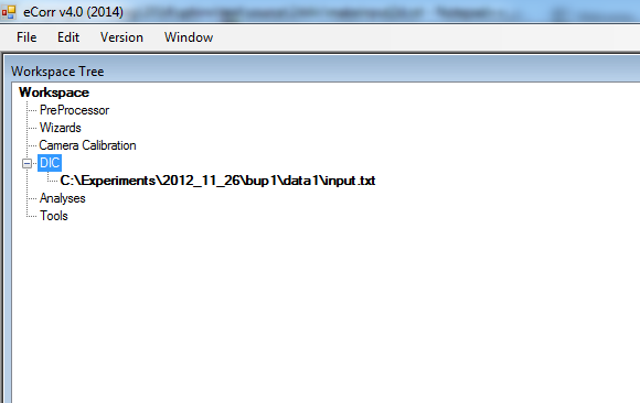
If you have run the edge-tracing analysis in a previous session, you can load the input file by right-clicking the “DIC” node in the Workspace Tree and choose “Load Input File...”. The input file will then appear as the image above.
Right-click on the input file in the Workspace Tree, and choose “Results View (image)” in the context menu.
The Results View (Image) will appear as shown below. The results viewer is linked to the specified input file. It is possible to open multiple result viewers for different input files.
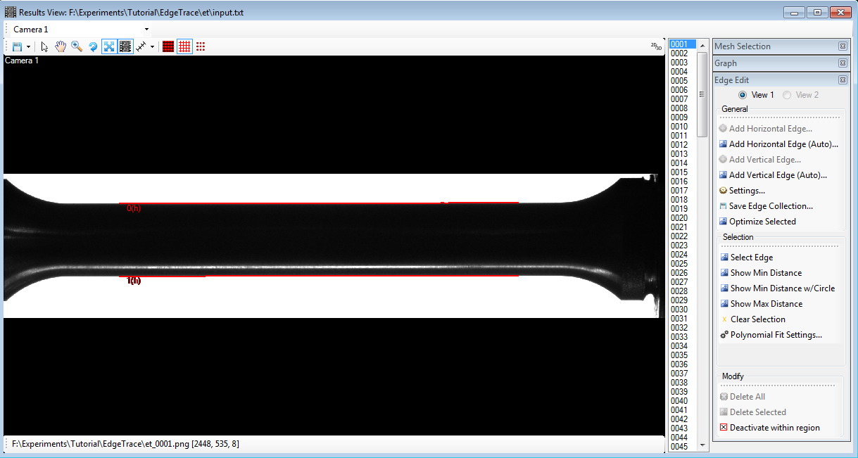
In the listbox to the right in the Results View (Image) , all the images in the current analysis are listed. You can decide which image to study by clicking in this list. By scrolling through the images in the list, you will see how the edge(s) has evolved from image to image.
The main features in the post-processing of the edge-tracing analysis is:
- Extract the minimum distance between edges as function of time
- Extract the curvature radius in the minimum-distance (necking-) region as function of time
Minimum Distance (Diameter)
First, the minimum distance may be visualized int the view by selecting Show Min Distance in the Edge Tool:
The minimum distance as a function of time can be plotted in a figure and/or exported to a text file.
To plot the minimum distance as function of time in a figure, open the Graph Tool. At the bottom of the tree-structure labeled “Available Data”, you will find the availabale data from the edge-tracing analysis under a node called Edges (Cam1):
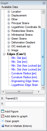
- Right-click on the Min. Dist [pix] node and select Set To Y-Axis. By default the X-axis is set to frame ID, but this can be changed.
Note
If more than two edges are present in the analysis, you will be asked which edge indexes to use in the minimum-distance calculation.
- Press the Add Data to Graph-button.
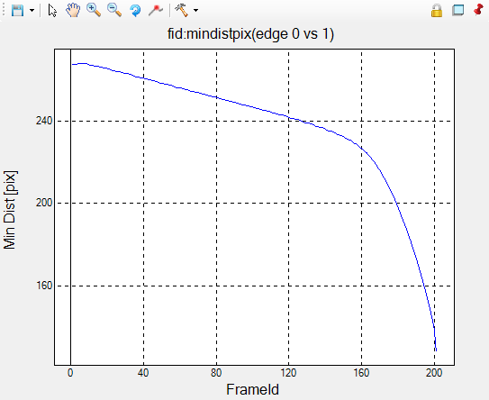
A Figure showing the temporal variation of the minimum distance will appear:
The minimum distance can also be written to a text file using the Export Data Tool:
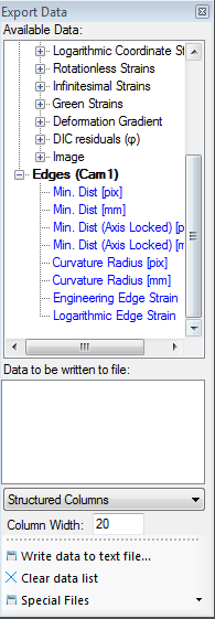
Similarly as for the Graph Tool, the available data from the edge-analysis is found at the bottom of the tree-structure labelled “Available Data”.
- First you may optionally add the frame ID as a column in the text file: Right-click the Frame-node at the top of the tree, and select Add Data to List.
- Right-click the Min. Dist [pix]-node and select Add Data to List.
- Press the Write Data to Text File-button.
- Choose a location for the text-file and press Save in the dialogbox that appears.
A text file are then written containing the minimum distance between the edges (in pixels). All data types added to the Data to be written to file-list, ends up as a column in the text file.
Hint
In order to access the minimum distance in millimetres (Min. Dist [mm]) a mm-per-pixel scaling factor must be added to the input file.
Curvature Radius
While the minimum distance is uniquely determined from the edge-tracing analysis, the curvature radius is not. The curvature radius is calculated using a Chebyshev polynomial fit in the results viewer.
The curvature-radius calculations used here, was published by Vilamosa et al.
- To acces the settings for the curvature radius calculations, choose Polynomial Fit Settings in the Edge Tool.
A dialog appears, which lets you define the settings for the polynomial fit:

An explanation of the calculations and the settings parameters above can be found here.
Note
Even though some default settings are provided for the curvature radius calculations, the settings should be manually adjusted by the user to get optimal results. The calculations are highly sensitive to poor settings parameters and the settings should be chosen with care.
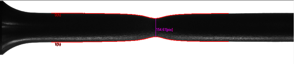
The curvature radius may be visualized by selecting Show Min Distance w/Circle in the Edge Tool:
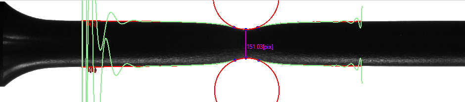
In the image above, the red curves are the edges found in the edge-tracing analysis. The green curves on the other hand, indicates the fitted polynomial. For both edges, there are three blue dots indicating the location of the minimum distance as well as the the closest locations (on both sides) where the second-derivative of the polynomial changes sign.
The two outer-most blue dots (for each edge) defines the boundaries of the region which are further used to optimize the circle. A circle is optimized to follow the edge in this region. The radius of this circle is then used as the curvature radius of the specimen.
To plot the curvature radius as function of time, open the Graph Tool.
- Right-click the Curvature Radius [pix]-node and select Set To Y-Axis.
You will now be asked for the indexes of the edges (even if there are two edges in the results). The curvature radius will be calculated for the edge indicated by the first index. Thus, if there are two edges in the view, select [0,1] to get the curvature radius for the first edge (index:0) and select [1,0] to get the curvature radius for the second edge (index:1).
- Press the Add Data to Graph-button.
A Figure showing the curvature radius for the particualar edge as function of time will appear:

What is important here, is that the radius calculations will not give sensible results for more or less straight edges. The necking of the specimen (and the corresponding edge) must be distinct before these calculations provide sensible results. Thus, it is the slope at the tail of the graph that is of interest.
If a curvature-radius graph from the point of necking until fracture is desired, the valid part of the curve in the figure above (inside red square) must be extrapolated backwards, as explained in Vilamosa et al.
The curvature radius can also be written to a text file, similarly as explained above for the minimum distance:
- Open the Export Data Tool.
- Right-click the Curvature Radius [pix]-node and select Add Data to List.
You will be asked for the edge indexes similarly as described above for plotting of the curvature radius. Remember that the curvature radius is calculated for the edge specified by the first index.
- Press the Write Data to Text File-button.
- Choose a location for the text-file and press Save in the dialogbox that appears.