Curvature Radius Calculations

The curvature-radius calculations used here, was published by Vilamosa et al.

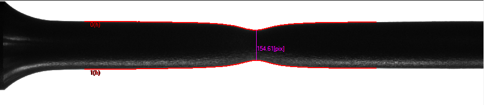
The curvature radius is calculated for a single edge, but two edges are needed to first find the location of the minimum distance (minimum diameter -> necking).

A Chebyshev polynomial with a specified degree is optimised (fitted) to follow the particular edge.

The settings for this polynomial fit can be accessed by selecting Polynomial Fit Settings in the Edge Tool:

If you want only a subregion of the edge to be part of the polynomial optimization, choose Use Clipping and specify a size of the clipping in pixels. If 100 pixels is chosen, 100 pixels to the left of the minimum-diameter location and 100 pixels to the right of the minimum-diameter location will take part in the polynomial fit optimization. The part of the edge that lies outside these boundaries are disregarded.

It is also possible to use weighting of the input to the polynomial fit optimization. If you choose Use Gauss Weighting, a Gauss-curve (bell-curve) with its center at the minimum-diameter location is used as weighting of the input. The specified distance in pixels gives the width of this bell curve.

Note

Even though some default settings are provided for the curvature radius calculations, the settings should be manually adjusted by the user to get optimal results. The calculations are highly sensitive to poor settings parameters and the settings should be chosen with care.

Below is an image showing the original edges in red, and the fitted polynomials in green. Note that because the Gauss weighting is activated, the polynomial fits the edges best close to the minimum-diameter location, while deviates heavily at the boundaries of the edges.

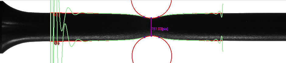
After the polynomial has been fitted, the locations where the second-derivative of the polynomial changes sign, closest to the minimum-diameter location, is found.

The minimum-diameter location as well as the these zero-second-derivative locations are indicated as blue dots in the image above.

The zero-second-derivative locations are further used as outer boundaries of the optimization of a circle.

A circle (center location and radius) is then optimized to fit the corresponding edge in the region limited by these zero-second-derivative locations.

The radius of the optimized circle is then used as the curvature radius of the specimen in the necking region.