Dimensional Splitting: Central-Difference Scheme (NT)
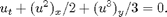
A test of dimensional splitting for the 2D scalar conservation law
Uses the second-order NT central scheme for the one-dimensional solvers. For more information, see front-tracking example.
Initial setup
xmin=-1.0; xmax=1.0;
T = 2.0;
N = 50;
h = (xmax-xmin)/N;
x = xmin:h:xmax; y = 0.5*(x(1:end-1)+x(2:end));
[X,Y] = meshgrid(y,y);
The initial function u0 is equal -1 inside a circle of radius 0.4 centered at (-1/2,-1/2), equal 1 inside a circle of radius 0.4 centered at (1/2,1/2), and zero otherwise. For later use, we define an anonymous function to do the computation of u0.
initData = (@(x,y) 1.0*((x+0.5).^2 + (y+0.5).^2 < 0.16) ...
   - 1.0*((x-0.5).^2 + (y-0.5).^2 < 0.16));
u0 = initData(X,Y);
contourf(X,Y,u0,-1:0.25:1); axis equal; colorbar, title('Initial data')

Number of time steps
In the first example, we fix the grid resolution and compare the approximate solutions generated with four different splitting steps (n=1, 4, 16, 64).
for i=1:4,
   tic;
   u=NTds(u0,y,y,'burger','cub',4^(i-1), T,'wbar','periodic');
   t=toc; st=sprintf('%4.2f',t);

   subplot(2,2,i);
   contourf(y,y,u,30), axis equal image; colorbar
   title( sprintf('Grid: %dx%d, Steps: %d', N, N, 4^(i-1)));
   xlabel(['Time used: ', st,' sec.']);
   p=get(gca,'position'); p([3 4])=p([3 4])+0.03;
   set(gca,'position',p,'XTickLabel',[]);
end

As was observed for the same problem with the front-tracking algorithm, it is amazing to observe how well the operator splitting method resolves the dynamics of the solution using only a few splitting steps.
Various grids
In the second test, we fix the CFL number to 20 and consider four different grid resolutions.
figure(2);
CFL=20;
for i=1:4,
   N= 32*(2^(i-1));
   h = (xmax-xmin)/N; delta=0.1/sqrt(N);
   x = xmin:h:xmax;
   y = 0.5*(x(1:end-1)+x(2:end));
   [X,Y] = meshgrid(y,y);
   u0=initData(X,Y);

   tic;
   Nstep=ceil(T/(CFL*h));
   u=NTds(u0,x,x,'burger','cub',Nstep,T,'wbar','periodic');
   t=toc; st=sprintf('%4.2f',t);

   subplot(2,2,i);
   pcolor(y,y,u), axis equal image; shading flat; colorbar
   title( sprintf('Grid: %dx%d, Steps: %d', N, N, Nstep));
   xlabel(['Time used: ', st,' sec.']);
   p=get(gca,'position'); p([3 4])=p([3 4])+0.03;
   set(gca,'position',p,'XTickLabel',[]);
end
