-
Week 2: Introduction, well-posedness
-
2008-01-09: Introduction, including a phase plane analysis of the system associated with the circular pendulum (section 1.1). I also touched a bit on sections 1.2–1.3.
2008-01-11: Chapter 1 from my notes (on well-posedness for ODEs). I also gave examples of non-uniqueness and of non-existence of solutions for an ODE with non-Lipschitz or non-continuous righthand side.
-
Week 3: The rest of Chapter 1.
-
2008-01-16: I finished what I wanted to say about well-posedness for (systems of) ODEs. I am sure everybody are greatly relieved! We will be much more practically oriented from now on. I covered sections 1.2–1.4, more or less. You may wish to look at 1.5 and 1.7–1.8 yourself.
2008-01-18: I was busy in a meeting, and Peter Lindqvist lectured in my place on linear 2×2 systems (by which I mean two equations, two unknown functions), i.e., sections 2.3–2.7.
-
Week 4: More on linearization and phase plane analysis.
-
2008-01-23: First a bit about a linear change of variables for linear systems. In the linear system ẋ=Ax (with x(t) a vector valued function, A a matrix) introduce new coordinates y by setting x=Vy, where V is an invertible matrix. One gets ẏ=V−1AVy, whose solutions are very easy to understand if A is diagonalizable, and V is chosen so V−1AV is diagonal. I showed how this would work out for 2×2 systems, then worked out some more details of the example in section 2.7 in the book, which had been started last Friday.
2008-01-25: More about linearization at equlibrium points in the plane. The theory is from Chapter 2 of my notes.
-
Week 5: Mostly finished chapter 2 of my notes, and of the book, started on chapter 3 in the book.
-
2008-01-30: Finished chapter 2 of my notes. I have also done some work on the 2×2 case of Chapter 3: At least I explained the 2×2 case of the rescaling argument that allows us to replace the 1 above the diagonal in (3.1) by ε and so leads to and estimate like (3.2). But the presentation of my argument suffered a bit at the end. Maybe we'll come back to it later.
I talked about Hamiltonian systems. Note that the book (only the 4th edition) has a bad misprint in the very definition of Hamiltonian system: There is a minus sign missing in the formula for Y (2.70) on page 75! (That minus sign makes a big difference.) Started on Example 2.11.
-
2008-02-01: Finished example 2.11 after getting lost in the wilderness of partial derivatives for a while. Note another mistake in the book: The arrows in Figure 2.13 are reversed.
Started on Chapter 3, with index theory.
-
Week 6: Chapter 3.
-
2008-02-06: More on the index of a point, including the theorem that the index of a curve is the sum of the index of each point inside it. I based the theory on that of homotopy rather than just using Green's theorem as in the book, but tried to keep it intuitive and not overly rigorous.
-
2008-02-08: Recalled that we have computed the index for all the linear systems with a non-degenerate matrix (all eigenvalues non-zero). The answer is −1 for saddle points and +1 for the others (foci, nodes, centers). What's more, the same is true for any zero of a smooth vector field: it has the same index as the linearization so long as no eigenvalues are zero. Showed some examples showing that the index of an equilibrium point can be any integer: Best described in a single complex variable as zk (index k) and its conjugate (index −k). Chapter 5 of my notes, on Bendixson's index formula.
-
Week 7:
-
2008-02-13: A bit about the behaviour of vector fields at infinity, and the index at infinity (section 3.2). Periodic orbits and limit cycles. I also explained a bit about Poincaré sections and the corresponding Poincaré map (section 13.1).
-
2008-02-15: More on periodic orbits, limit cycles, and Bendixson's negative criterion (plus Dulac's variant) (section 3.4). Homoclinic and heteroclinic orbits (section 3.6).
-
Week 8: Quoting Monty Python: And now for something completely different. Namely, Fractals and chaos. I intend to spend no more than two weeks on this break from the main focus of the course.
-
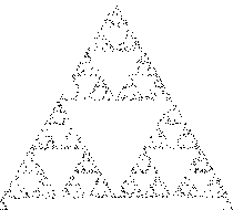
2008-02-20: Mostly on iterated function systems (IFS) and how they define fractals. I showed one way to generate fractals via a random iteration on the IFS: The first picture here shows the top 1/9th of the Sierpinski triangle after 111110 iterations and the second, after 1111110 iterations. I put together a simple animation showing the state after 10, 110, 1110, 11110, 111110 and 1111110 iterations. (The source code is available for the morbidly curious.)
-
2008-02-22: Fractal dimension. This lecture was only an hour (45 minutes really) long. I defined the fractal dimension, computed it for the Cantor set and the Sierpinski triangle, and wrote up the general formula for a fractal generated by similitudes and verified that it produced the same answer for our two examples.
-
Week 9:
 Finished the chaos and fractals note. Among other things I proved the chaotic nature of the map on [0,1] that maps 0 and 1 to 0, 1/2 to 1, and is linear in between.
-
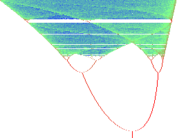
2008-02-27: Started on chaos, including some numerical experiments on the Verhulst mapping. (Two larger versions of the picture on the right – and explained in the notes: just plain bigger, and zoomed vertically to make more details visible.) I also discussed the definition of chaos as given in the notes.
-
2008-02-29: Proved that the piecewise linear system on [0,1] as described in the notes is in fact chaotic. Then we returned to the book (Chapter 8), with a discussion of Poincaré stability and Lyapunov stability as applied to non-constant solutions for a dynamical system.
-
Week 10: No lectures.
-
Week 11: No lectures.
-
Week 12: Easter week. No lectures.
-
Week 13: We continue in Chapter 8.
-
2008-03-26: More on Poincaré and Liapunov stability (8.1–8.3), including an example from which I recklessly generalized the conjecture that a stable limit cycle is “usually” Liapunov stable. (By which I mean that, if it is sufficiently stable that nearby orbits converge exponentially to the limit cycle, then Liapunov stability should follow.)
Chapter 4 from my notes on linear systems with variable coefficients, which is just a super efficient way of doing what sections 8.5+8.6 in the book does more slowly. (But have a look at what the books says too.)
-
2008-03-28: First a remark on how the fundamental matrix Φ(t) is essentially unique in the sense that any other fundamental matrix can be written Φ(t)B where B is a constant invertible matrix. Then sections 8.7 and 8.8. I went a bit further then the book for section 8.8, considering the Jordan form and showing that stability is equivalent to having the real parts of all eigenvalues ≤0, plus having equal algebraic and geometric multiplicities for all eigenvalues with real part =0. (My “proof” was basically a lot of hand waving in the case of complex eigenvalues, but almost complete for the case of real eigenvalues.)
-
Week 14: We have work left to do in Chapter 8, but I'd rather use the proof method from my notes, and that requires a peek at the Liapunov method for evaluating stability first. So we'll dive into Chapter 10.
-
2008-04-02: Chapter 10: I basically did section 10.6, but formulated for n=2. Thus we also covered the theory needed for 10.1–1.04, but without the topographic systems that are used so heavily in those sections (I don't quite see the point). We also leave the Poincaré–Bendixson theorem for later. I also did a variant of section 10.5: If there is a weak Liapunov function and it is not constant on the forward half of any phase path, then the equilibrium is asymptotically stable.
-
2008-04-04: Peter Lindqvist lectured from Chapter 3 of my notes. That can be used as a substitute for sections 8.9–8.11 in the book. I have made a small addition to the note on page 18, that can serve as a replacement for section 8.10.
-
Week 15: The Hartman–Grobman theorem and the Poincaré–Bendixsson theorem
-
2008-04-09: In the first half, I stated (but didn't prove) the Hartman–Grobman theorem and explained its strengths and weaknesses (end of Ch 3 in my notes). In the second half, I laid some of the groundwork for the Poincaré–Bendixsson theorem (Ch 6 in my notes) including an example showing that the theorem as stated in the book is wrong.
-
2008-04-11: I (more or less) proved the Poincaré–Bendixsson theorem and gave an example of its use.
-
Week 16: (Only three weeks of lectures left.)
Sections 11.1–11.4., starting with Liénard equations are in 11.1.
-
Week 17: (Last week with new material.)
Sections 12.1–12.4, on bifurcations. For the saddle-node bifurcation, I explained the middle picture on p. 413 by a rescaling of the variables x, y, using instead the variables X, Y defined by x=√(μ)X, y=μY and noting that the vector field has a fast and a slow component, where the fast, vertical component vanishes on the “slow” curve Y=X2−1. Also, the transcritical bifurcation turns into a saddle-node bifurcation (actually two copies of the right half plane) by replacing x by x+μ (or something like that; I changed the equation a little bit to make that work better).
-
Week 18: Summary, highlights.