Logarithmic Strains
In a 2D-DIC analysis, a two-dimensional displacement field  is measured. Here
  denotes a position in the reference coordinate system.
 denotes the time, usually associated to the image ID in a sequence of images.
For any position and any time the two-dimensional deformation gradient may be calculated as:

The two-dimensionalright Cauchy- Green deformation tensor  is then calculated as:

The in-plane principal streches  are found by solving the eigenvalue problem for the right Cauchy-Green deformation tensor:
where  , the eigenvectors, gives the principal directions of the right Cauchy-Green deformation tensor.
Note
Because of the two-dimensional nature of the DIC measurements, the third principal direction  is assumed to be normal to the surface of the specimen, i.e. the shear strains through the thickness of the specimen are assumed negligible.
The in-plane principal logarithmic strains are then calculated from the principal stretches:

where the rotation of the principal strains is given by the eigenvectors .
Note
In eCorr it is also possible to obtain the third principal strain component  , i.e. through the thickness. However, this is only valid where we can assume negligible elastic strains and plastic incompressibility.
Then, the third component is estimated as follows:
, i.e. through the thickness. However, this is only valid where we can assume negligible elastic strains and plastic incompressibility.
Then, the third component is estimated as follows:  .
.
Further, an effective strain measure  based on the von Mises norm is available. This is defined as

A two-dimensional strain matrix is established using the calculated principal strains:
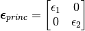
Now, this principal strain matrix  is associated with the principal directions .
To obtain the strain matrix for a specific direction, the matrix may be rotated using a two-dimensional rotation matrix
is associated with the principal directions .
To obtain the strain matrix for a specific direction, the matrix may be rotated using a two-dimensional rotation matrix  :
:
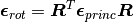
Thus, by using the rotation provided by the principal directions , the strain matrix can be rotated back to the coordinate domain, giving the logarithmic coordinate strains:

Note
When time-series of strains are plotted or exported in eCorr, the strains are always calculated in the center of an element.