
Faculty of Medicine and Health Sciences
Department of Circulation and medical imaging
Strain rate imaging.
Revised edition
Basic concepts of motion and deformation
by
Asbjørn Støylen, Professor, Dr. Med
asbjorn.stoylen@ntnu.no
This section:
Deals with the basic concepts of motion (displacement and velocity) and deformation (strain and strain rate), and how these concepts are related to myocardial deformation, and inter related.
This section replaces the two old sections:
- Basic concepts of motion and deformation
- Basic concepts in myocardial strain and strain rate
- Motion versus deformation
- Relations
between velocities and strain frate
- Velocity gradient
- Longitudinal velocity gradient (strain rate)
- Is there a gradient of strain and strain rate from base to apex as well?
- Velocity
and strain rate
- Displacement and strain
- Differences between
walls
- Strain rate and strain
- Strain in three dimensions
- Left ventricular myocardial systolic strains
- Properties of the different strain components
- Absolute longitudinal LV shortening is Mitral annular motion (MAPSE)
- Relation between systolic longitudinal ventricular shortening / MAPSE and stroke volume
- Longitudinal
strain/ Relative shortening
- Transmural strain
- Circumferential
strain
- 1:
Circumferential strain equals diameter shortening
- 2: There is a gradient of circumferential strain from outer to inner surface
- 3: Only outer circumferential strain is a function of circumferential fibre shortening, both the midwall and endocardial circumferential strains as well as the gradient are mainly a function of wall thickening.
- Area
strain
- Regional strain and strain rate
- Segmental strain with other segments interact through both contractility and load.
- Regional MAPSE cannot identify infarct site, only infarct size
- Segmental
shortening is also changed by asynchronous
shortening, even in normal contractility
- Right ventricular strain
Motion and deformation
Fundamentally, an object has motion if it changes position, and deformation if it changes shape. Displacement and velocity are motion. A stiff object may move, but not deform. A moving object does not undergo deformation so long as every part of the object moves with the same velocity. An object that deforms may not move in total relative in space, but different parts has to move in relation to each other for the object to deform. The object may then be said to have pure translational velocity, but the shape remains unchanged. Over time, the object will change position – this is displacement. Velocity is a measure of displacement per time unit.
Of the four objects shown here, A is stationary and has neither motion nor deformation. B moves, i.e. it has motion, but the length remains the same, so the object is not deformed. The two ends of the bar move with the same velocities. C is stationary (at least one end), but the other end moves, so the length increases, the object is deformed. In D, all parts of the bar moves. but with different velocities, so in additionto motion, the object also lengthens, i. e. it is deformed.
which describes deformation relative to baseline length, where


Strain rate. Both objects show 25% positive strain, and both corresponds to the object above, but with different strain rates, the upper has twice the strain rate of the lower. If the period is one second in the upper object, the strain rate is 25% or 0,25 per second, giving a strain rate of 0.25 s-1. The lower object has twice that period, i.e. half the strain rate, which then is 0.25 / 2 seconds = 0.125 s-1 . In both cases, the strain rate is constant.
If the strain is constant, as in the example above, the strain rate is strain per time unit, which is equal to change in length per time , and this again to velocity per length:
Strain and strain rate
as numerical versus signed values
As we see, the Lagrangian (and Eulerian too) definition of strain is mathematical, where dimension increase (lengthening) is positve strain and strain rate, and dimension decrease (shortening) is negative strain, i.e. strains are given by signed numbers.
In the heart, however, strain is mainly used for systolic deformation. In systole, the ventricles shorten longitudinally and circumferentially, while the walls thicken, i.e. in systole:
- Longitudinal shortening is decreasing length = negative strain
- circumferential shortening, is decreasing circumference = negative strain
- transmural thickening, is increasing thickness = positive strain
When viewed as coordinates of ventricular deformation in three dimensions; longitudinal, circumferential and transmural strain, the interrelation makes the mathemathically correct version the most useful and appropriate.

Also, the volume deformation of the ventricular myocardium relates to the strain components whenn using the signed strain values:
If, on the other hand
as a numerical measure,
Likewise, in the whole ventricle, looking at dimension and volume changes, most volume changes are defined in the positive domain:
MAPSE is the most used measure of absolute longitudinal shortening and is positive, as both motion and velocity towards the prove are defined as positive, thus following the Doppler conventions..
Fractional diameter shortening is numerically equal to circumferential shortening, but defined as: FS = (DD - DS) / DD (although this definition is also arbitrary, FS = (DS - DD) / DD, giving diameter decrease as negeative.), which is positive.
SV is a positive measure of absolute stroke volume, although the definition SV = LVEDV - LVESV could just as well have been reversed (SV = LVESV - LVEDV), defining volume decrease as negative. .
,EF, whichb is relative volume decrease, is defined as EF = SV / LVEDd, and is thus a positive measure, but again this is arbitrary, and might be reversed.
For physiological considerations, increased contraction, meaning higher MAPSE, FS, SV, EF, might be matched by "more or higher relative shortening". Relative shortening is also more useful for direct comparison of longitudinal relative shortening, as we did in the later HUNT3 studies (18, 23) when comparing MAPSE and S' with normalised MAPSE and S' as well as GLS and GLSR.

Velocity imaging. Parametric (colour) image. In this parametric image all carriages that are in motion (have velocity) are coloured red, carriages with no motion (zero velocity) have no colour.
The engine starts first, then the carriages are successively brought into motion. When all carriages are in motion, the train runs evenly, and all carrriages are red. In stopping, the engine stops fist, then the carriages stop sucessively, until all carriages are motionless. However, both at standstill (the whole train is white) and running evenly (whole train red), there is no deformation, only motion. The deformation occurs when any two carriages are moving with different velocities. This is shown below.

Deformation imaging. Parametric (colour) image. This is the same figure as above, but in this image, the two carriages with different velocities are shown in either cyan (stretching) or orange (compression), while the other carriages where no deformation occurs (whether running evenly or standing still) are shown in green. When the train is immovable, there is no deformation, the whole train is green. As the engine starts, there is stretching between that and the first carriage (cyan). Once the first engine is at the same velocity as the engine, no further stretching (deformation) of that connection occurs, while the stretching has moved backwards in the train to the next connection. The stretching can be seen as a wave of deformation (cyan) moving backwards in the train. (Another example of this is given in the section on diastolic strain rate). Once all carriages move with the same velocity, no further deformation occurs, and the whole train has even motion, and is coloured green again. When all parts of the object have the same velocity, there is no deformation. In stopping the opposite occurs, there is compression between engine and first carriage, then between first and second carriage, and so forth. The compression can be seen as an orange wave moving backwards through the train. When the train is at standstill, no further deformation occurs. When different parts of the object have different motion, there is deformation of the object. Deformation is thus differential motion.


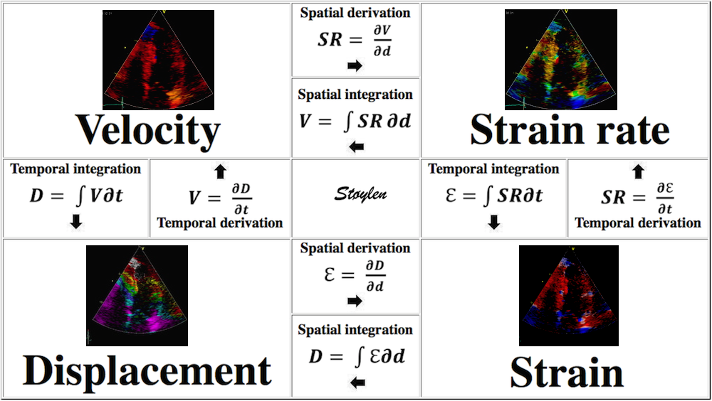
Derivation and
integration
Since velocity is the temporal derivative of displacement (the rate of displacement):
and strain rate is the temporal derivative of strain (the rate of deformation):
Displacement, velocity, syrain and strain rate are all related through spatial and temporal derivation and integration:
During a heart cycle the base of the ventricles moves towards the apex in systole, and away from apex during early diastole and atrial systole. This means that both motion and deformation varies through the heart cycle.

As the base moves towards the apex in systole, and away from apex in diastole, the LV base (and all other parts of the LV) has positive motion in systole, negative in diastole. But as the motion decreases towards zero from base to apex, the ventricle has negative strain and strain rate during systole, positive strain rate during diastole.
The cardiac apex is known
to be stationary, except for the small motion felt as the
apex beat, which is well known as a clinical event. This
motion is towards the chest wall. The apex is
pressed forwards and collides with the chest wall during
systole, and marks the location of the cardiac apex on
clinical examination. The apex beat has been shown to be a
systolic event, by apexcardiography (10),
and the real motion is minimal.
 |
 |
 |
| The apex beat, shown here in an apexcardiogram recorded with a pressure transducer, demonstrating that the beat is a systolic event. (Image modified from Hurst: The Heart). | The apex beat can
also be demonstrated by tissue Doppler, yellow:
Base, cyan: apex. |
and by integrating
the velocity curve,
the apical displacement (green curve) can be
seen to be minimal |
Looking at the myocardial motion, it is evident that apart from the apex beat, the apex is nearly stationary, while the ventricular basis moves towards the apex during systole. This was demonstrated already by Leonardo da Vinci (11), and confirmed by various methods (12 - 15).
 |
 |
| As the apex is nearly stationary, while the base moves toward the apex in systole, away from the apex in diastole, the ventricle has to show differential motion, between zero at the apex and maximum at the base. Longitudinal strain will be negative (shortening) during systole and positive (lengthening) during diastole (if calculated from end systole). | M-mode lines from an
M-mode along the septum of a normal individual.
These lines show regional motion. It is evident
that there is most motion in the base, least in
the apex. Thus, the lines converge in systole,
diverge in diastole, showing differential motion,
a motion gradient that is equal to the deformation
(strain). |
Tethering

In this image we see the train moving along. Both the engine and the coaches have motion as seen by the red colour, but only the engine has intrinsic motion, the coaches are tethered to the engine imparting motion to them by pulling them along.
A myocardial segment may move due to being tethered to a neighboring segment. As every segment has local shortening (strain), they will also affect other segments, pulling them, along . In the longitudinal direction, this means that the apical segments shortens, pulling the midwall and basal segments along, imparting motion. Likewise will the midwall segments shorten, imparting even more motion to the basal segments. This is the basis for the longitudinal velocity gradient.
Physiological tethering
As every segment has local shortening (strain), they will
also affect other segments, pulling them, along (tethering).
In the longitudinal direction, this means that the apical
segments shortens, pulling the midwall and basal segments
along, imparting motion. Likewise will the midwall segments
shorten, imparting even more motion to the basal segments.
This means that the apical segments shows corresponding
motion and shortening, while the midwall segments show
motion from intrinsic shortening, plus motion imparted from
being tethered to the apical segments, and the basal
segments shows motion from intrinsic shortening, plus motion
imparted from the shortening of both apical and midwall
segments by the tethering. This is the basis for the longitudinal
velocity gradient. |
 |
| MOdel of the left
ventricle, where the length is divided into only
two levels, apical and basal. The segments in
both levels develop tension, leading to
shortening (deformation) in both apical and
basal levels. The shortening of the apical
levels (orange arrows), in addition to
deforming, will also pull the basal segments in
the apical direction. The basal segments, in
addition to moving, will also shorten (green arrows),
so the base of the heart (yellow) moves more
than the midwall (cyan), which moves more than
the apex (red). |
Actual curves from
septum of a healthy subject, showing equal
shortening of the apical (orange curves) and
basal (green curves) segments. This shows how
the base (yelllow) moves more than the midwall
(cyan) which moves more than the apex (red). |
Thus, the normal state is that the apical segments have deformation, while the midwall and base have increasing motion by being both tethered, as well as being actively deforming as well.
Tethering as source of
motion in passive segments
The point of tethering is also that a passive segment
is tethered to an active segment, and thus is being pulled
along by the active segment, without intrinsic activity in
the passive segment: |
 |
 |
| A patient with an inferior infarct.
Tethering: The basal and midwall segments are
infarcted, and are stiff, but being pulled along
by the active apical segment. |
Velocity
curves. All of the wall has motion,but as the
midwall and basal segments follow the exct
same velocity curve as the apical segment, it
is evident that they are tethered, as the
coaches above. However, as the whole wall has
motion, this must be from the apical segment,
acting as the engine and pulling the rest of
the wall along. |
And the motion
shows the same thing, passive motion in base and
midwall, being tethered to the active apical
segment. |
Looking at deformation instead, pure motion due to tethering will not have deformation:

In this image we see the train moving along. As the whole train moves by being tethered to the engine's intrinsic motion, there is no deformation, as seen by the green colour.
|
 |
 |
| Strain rate
(unsmoothed). The curves show no deformation in
the base (yellow), some deformation in the
midwall (cyan) and normal deformation in the
apex (red). |
Strain curves, showing the same as strain
rate. Basically, this shows the apex to be the
active segment, in an easier way thatn by the
mnotion curves. |
This means that a passive segment may show motion, but without intrinsic deformation, and the deformation imaging will discern that. This is evident both in systole and diastole.
The whole heart
cycle
During the heart cycle, the ventricle shortens in systole, and elongates during early and late filling phases, This means that the different measures change during the heart cycle, and the motion is largest in the annular plane, and varies between the walls.
Lagrangian and Eulerian strain
There are two different ways of describing strain and strain
rate: Lagrangian and Eulerian (named after the two
mathematicians Joseph-Louis Lagrange and Leonhard Euler,
respectively.
Lagrangian strain is the strain defined above; ![]() the change in length divided by the
original length, while Eulerian strain is the strain divided
by the instantaneous length;
the change in length divided by the
original length, while Eulerian strain is the strain divided
by the instantaneous length; ![]() .
.
Some prefer to use the term "Natural strain" instead of
"Eulerian". I'm no fan of I fail to see how one reference
system is more "natural" than another. Using both
mathematicians' names, the nomenclature will at least be more
symmetrical.
 |
 |
| Lagrangian strain
(top) and Eulerian strain (below). Visually, it is
evident that both objects undergo the same strain at
the same strain rate. Thus, the physical reality is
the same, but the two figures show the two different
ways of describing the deformation, as the
Lagrangian strain shows an increasing deformation
relative to the constant baseline length, while
Eulerian strain describe the deformation (in this
case constant, as the strain rate is constant, but
this is not a condition), relative to the
continually changing length. |
Lagrangian strain
(top) and Eulerian strain (bottom). Only four point
in time is shown, to illustrate how this means that
by Lagrangian strain at any time is the sum of all
length increments up to that time, divided by the
baseline length, while Eulerian strain at any time
is calculated as the sum of all ratios of length
increments and the instantaneous length up to the
actual time. |
Thus, as described above left, Lagrangian strain is the
cumulated deformation, divided by the initial length:
Eulerian strain is the cumulated ratios between the instantaneous deformation and the instantaneous length:
![]()
The point is that the two formulas will result in slightly different values. The positive Lagrangian strain of 25% in the example above, will be equivalent to 22% Eulerian strain (and not 20%, as one might believe). In general, peak strain may be up to 4% higher (absolute values but a relative difference of up to about 20%) by Eulerian strain than by Lagrangian strain.
 |
 |
| Lagrangian versus Eulerian strain. Lagrangian strain will give slightly higher values, i.e. negative strain values are lower absolute, while positive values are higher. |
Strain curves as seen below.
Lagrangian and Eulerian strain curves. As
myocardial strain in general is negative, the
Eulerian strain curve lies below the Lagrangian. |
or at any given time
However, in continuous moving material points through spatial points, i.e. continuous deformation, the Eulerian strain is exact only when the increments and time intervals are small, i.e.:

The relations between Eulerian and Lagrangian strain rates are:
Relation between velocities and strain rate
Velocity gradient
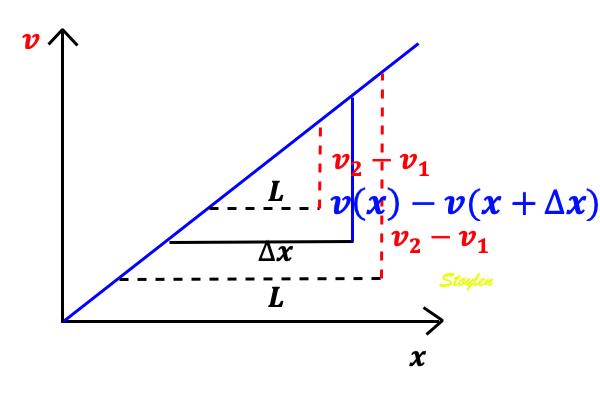
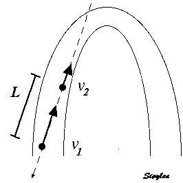
The velocity gradient is the slope of the velocities along the the object. If velocities are linearly distributed through the object, this is equal to the difference in the end velocities, divided by the instantaneous Length (L):
Velocity gradient. There are different velocities in the two ends 1 and 2, and if velocities are evenly distributed along the object, the velocity gradient is equal to the difference between the velocities at the end, divided by the instantaneous length. As v1 > v2, in this case VG is negative, and the two points approach each other, i.e the object shortens.
As SR is the spatial derivative of the velocities,
Then SR equals the velocity gradient if the velocities are evenly distributed:
The distance L changes with time, if v1 and v2 are different. The unit of the velocity gradient is cm/s/cm, which is equal to s-1. But as the the velocities of the two points is the displacement per time:
then the velocity gradient equals the Eulerian strain rate.:
And the time integral of the velocity gradient equals Eulerian strain:

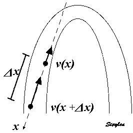
Measuring the deformation of a segment. The segment is defined by the end points x and x+
In this case, it is evident that in the changing L, the velocities change simultaneously, keeping the ratio between the differences and the instantaneous length constant (0 the slope). This is also the case for the ratio between the difference in velocities, v(x) - v(x +
Longitudinal velocity gradient (strain rate)
The concept of velocity
gradient was introduced by Fleming
et al (20),
defined as the
slope of the linear regression of
the myocardial velocities along the
M-mode line across the myocardial
wall. If velocities are linearly
distributed through the wall, this
is equal to the difference in
endocardial and epicardial
velocities divided by the
instantaneous wall thickness (W):
The definition of transmural velocity gradient was extended by Uematsu (21), by applying the velocity gradient to wall thickening velocity in any direction in the 2D cross sectional image, by means of angle correction of the velocities.
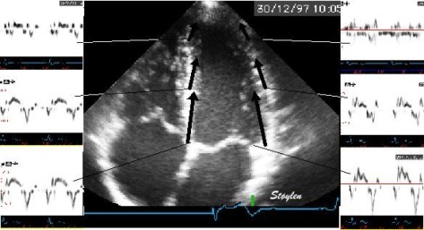
As the apex is stationary, while the base moves, the displacement and velocity has to increase from the apex to base as shown below.
 |
 |
|
| As the apex is stationary, while the base moves toward the apex in systole, away from the apex in diastole, the ventricle has to show differential motion, between zero at the apex and maximum at the base. | As motion decreases from apex to base, velocities has to as well. This is seen very well in this plot of pwTissue Doppler recordings showing decreasing velocities toward apex. Thus, there is a velocity gradient from apex to base |
The simultaneous measurement of velocities by colour Doppler in the whole sector, enables the measurement of instantaneous velocity differences.
At the NTNU, Andreas heimdal was working with deformation imaging, while I was working with long axis left ventricular function at the same time. This led to me suggesting to apply the velocity gradients to the longitudinal shortening, which are greater in magnitude, making the rough method more robust, as well as making all segments of the ventricle available for analysis, and resulted in the first publication on strain rate imaging (22).
 |
 |
| The strain rate can be described by the instantaneous velocity gradient, in this case between two material points, but divided by the instantaneous distance between them. In this description, it is the relation to the instantaneous length, that is the clue to the Eulerian reference. | Strain rate is calculated as the velocity gradient between two spatial points. As there is deformation, new material points will move into the two spatial points at each point in time. Thus, the strain that results from integrating the velocity gradient, is the Eulerian strain. |
The strain rate was calculated as the velocity difference between two spatial points, divided by the distance between them, but as shown above, this is equivalent to the velocity gradient, and thus to Eulerian strain rate.
Is
there a gradient of strain and
strain rate from base to apex as
well?
The velocity gradient from base of the LV to the apex looks fairly linear:
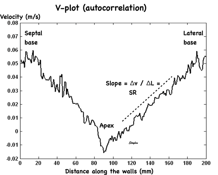
Peak systolic velocity plot through space, from the septal base to the left through the apex in the middle to the lateral base to the right. The velocities seem to be distributed along fairly straight lines, i.e. there seems to be a fairly constant velocity gradient.
Thus, while peak velocities decrease, peak strain rate is more or less constant from base to apex if the gradient is constant.
It has been maintained that as the curvature is larger (smaller radius both in cross sectional and longitudinal planes) in the apex, the wall stress (i.e. load) is lower, and hence shortening higher, in accordance with the law of Laplace. However, this reasoning do not take the varying wall thickness into account. As the wall is thickest at the base, and thinnest at the apex (46), the wall thickness decreases as the radius decreases, and no conjectures about the wall stress can be made.
Some of the earliest strain rate studies found no base - to apex gradient (47 - 49), although later studies seem to find differences with lowest values in the apex (50). However, in that study, the greatest angle error was also in the apex (51).
This was also found in the HUNT3 study (17) of 1266 subjects without indications of heart disease.
Peak systolic segmental strain and strain rate by combined tissue Doppler and speckle tracking of segmental borders, according to ventricular levels, the full material
| Basal |
Mid
ventricular |
Apical |
Total |
|
| Peak
systolic strain rate (s-1) |
-0.99
(0.27) |
-1.05
(0.26) |
-1.04
(0.26) |
-1.03
(0.13) |
| End
systolic strain (%) |
-16.2
(4.3) |
-17.3
(3.6) |
-16.4
(4.3) |
-16.7 (2.4) |
Looking more closely at the segmental velocity gradients per se by method comparisons (N=57), there was lower numerical values in the apex, but only only when the ROI did not track the myocardial motion through the heart cycle. Tracking the ROI eliminated this gradient, indicating that this was artificial.
With speckle tracking, some authors have found a reverse gradient of systolic strain as well, highest in the apex (52, 53). However, in that application, measurements are curvature dependent, the curvature being highest in the apex and lowest in the base, and the discrepancy between ROI width and myocardial thickness being greatest.
Interestingly, a recent study looking at aortic stenosis, fond an apex to base gradient in the most severe cases (reduced in the base), but no gradient in the less pronounced cases (54). An even more pronounced finding is described in a study of apical sparing in amyloidosis (55), with no gradient in the two reference populations: Normals and hypertensive controls as a hypertrophic reference group without amyloidosis
This, by corollary, should also be a case for no gradient in the normal state. Thus, the base to apex gradient may be a result of the speckle tracking software combined with the processing.
In the method comparison in the
HUNT3 study (N=57) (19),
taking care to avoid both
foreshortened images and excessive
curvature, there were no level
differences in 2D strain either:
| Segment
length by TDI and ST |
2D strain
(AFI) |
|||
| Peak
Strain rate |
End
systolic Strain |
Peak Strain rate | End systolic Strain | |
| Apical | -1.12
(0.27) |
-18.0
(3.6) |
-1.12
(0.37) |
-18.7
(6.6) |
| Midwall |
-1.08
(0.22) |
-17.2
(3.2) |
-0.99
(0.23) |
-18.3
(4.7) |
| Basal |
-1.03
(0.24) |
-17.2
(3.5) |
-1.12
(0.36) |
-18.0
(6.2) |
| Mean |
-1.08
(0.25 |
-17.4
(3.4) |
-1.07
(0.33) |
-18.4
(5.9) |
In this case care was taken to align ROI shapes as much as possible.
MR tagging studies have also found
various results. Bogaert and
Rademakers (56)
in a study of healthy subjects
(N=87) found lowest longitudinal
strain in the midwall segments,
higher in both base and apex, but no
systematic gradient from base to
apex. Moore et al (57)
in a study of healthy volunteers (N=
31) found a systematic gradient, but
with the lowest
strain in the apex, highest in
the base. CMR feature
tracking have not found
convincing base to apex gradient
either (31,
58).
Thus, it seems that the velocity
gradient from base to apex is
linear, and that there is no
gradient of neither strain rate nor
strain from base to apex, as
illustrated below:

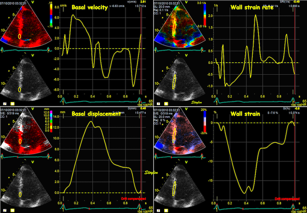
Top left: Velocity curves from four different points of the septum. The image shows the evenly decreasing velocities from base to apex. Top right: the resulting strain rate curves from the segments between two and two of the velocity ROIs displayed. Bottom left: Displacement curves from the same four different points of the septum, obtained by integration of the velocity curves. The image shows the evenly decreasing displacement from base to apex. The resulting strain curves from the segments between two and two of the velocity ROIs shown to the right.
The velocity gradient is also very
evident when velocities are derived
by speckle tracking:

Velocity
and strain rate
We have shown above
that strain rate (velocity gradient)
is equal to the spatial derivative
of the velocity, which is velocity
difference per length:

Thus the distance between the two curves is an indication of the strain rate:

But this means, the apex being nearly stationary, that the global strain rate (of a wall or the whole ventricle), equals the normalised, inverse value of the annular velocity: the annular velocity corresponds fairly closely to the wall strain rate (23).
|
 |
| As we see, apical velocity is close to zero. | When strain rate (SR) is taken from tissue velocities, the definition is SR= (v(x) - v(x+Δx)) ⁄ Δx where v(x) and v(x+Δx) are velocities in two different points, and Δx is the distance between the two points. If the two points are at the apex and the mitral ring, the apical velocity v(x) ≈ 0, apex being stationary, and v(x+Δx) is annular velocity. Δx then equals wall length (WL), and peakSR = (0 - S') ⁄ WL= (-S') ⁄ WL. |
If the two points are
at the apex and the mitral ring, the
apical velocity ![]() , apex being
stationary, and
, apex being
stationary, and ![]() is annular
velocity.
is annular
velocity. ![]() then equals wall
length (WL),
then equals wall
length (WL),
thus ![]() and
peak
and
peak ![]() . It's also evident
that the basal velocity curve and
the strain rate curve approaches
each other's shape when strain rate
is sampled from most of the wall
length. Thus,
peak strain rate is peak annular
velocity normalised for wall
length.
. It's also evident
that the basal velocity curve and
the strain rate curve approaches
each other's shape when strain rate
is sampled from most of the wall
length. Thus,
peak strain rate is peak annular
velocity normalised for wall
length.

When strain rate is sampled from most of the wall length, the shape is close to an inverted version of the basal velocity curve.
However, This is when strain is calculated over a whole wall. Looking at the curves at the top of this section, we see that the velocities peak earlier than strain rate.


Strain rate is the difference between the curves. Here the difference between the two velocity curves is calculated in excel (red) without the length correction, (which then is equal to SR*1.2). As can be seen, the early steep slopes of both curves (orange) will result in a much less steep slope in the difference curve, as they diverge very little from each other. From the peaks of the velocity curves the two curves seem almost parallel, despite both dipping sharply, this results in a near horisontal strain rate curve, and finally the slow convergence of the curves give a much slower reduction of the difference.
Looking at the basal half of the septum, there is an early peak in both basal and midwall velocity curves (yellow and cyan), while the apical curve (red) is flat. Looking at the strain rate curves, the basal half shows a rounded curve (green) with later peak, while the apical half shows an early peaking strain rate curve (orange), closely resembling an inverted velocity curve. This, of course corresponds to the velocity differences shown by the corresponding areas between them, the basal and midwall curves have parallel early peaks, and thus there is no strain rate peak between them, the maximum difference is actually in mid systole, the midwall curve shows a peak, the apical is flat, and thus there is a corresponding early peak in the strain rate curve.
Displacement and strain
Exactly the same is the case for basal displacement vs strain, of course.

Thus the distance between the two curves is an indication of the strain.
As the apex is near stationary, the displacement of the mitral annulus is the shortening of the whole ventricle: and the shortening divided by the length of the ventricle or walls is a measure of the the global strain.

|
 |
| The same as for velocity vs. strain rate, of course, must then hold for displacement vs strain. | Likewise, strain = (d(x)-d(x+Δx)) ⁄ Δx where d(x) and d(x+Δx) are displacements in two different points, and Δx is the distance between the two points. If the two points are at the apex and the mitral ring, the apical displacement d(x) ≈ 0, apex being stationary, and d(x+Δx) is annular displacement = MAPSE. Δx then equals wall length (WL), and Strain = (0-MAPSE) ⁄ WL= -MAPSE ⁄ WL. When strain is sampled from most of the wall length, the shape is close to an inverted version of the basal displacement curve. |
Longitudinal systolic strain and MAPSE have been shown to have a close correspondence (18).
Differences between walls
Both MAPSE and peak systolic velocity vary normally between walls (16, 98, 99), but the average of lateral wall and septum is very close to the average of four or even six walls within the limit of measurability (7, 16, 18, 19, 99).
In the HUNT study, the same differences were found in systolic annular velocities, with differences between septum and lateral wall of the order of 10% (16), but not in deformation parameters (17), where the same difference was on the order of 4% in strain rate and only 1% (relative) in strain:
Normal annular peak systolic velocities, strain rate and strain per wall in the HUNT3 study by tissue Doppler.
Values are mean values (SD in parentheses). Velocities are taken from the four points on the mitral annulus in four chamber and two chamber views, while deformation parameters are measured in 16 segments, and averaged per wall. The differences between walls are seen to be smaller in deformation parameters than in motion parameters, although still significant due to the large numbers.
The displacement and peak systolic
velocity is higher in the lateral
wall than the septum, while
deformation is much more similar in
the different walls, being
normalised for the wall lengths:

Colour
Doppler traces of velocity,
displacement, strain and strain
rate from the septal (yellow)
and lateral (cyan) aspect of the
four chamber view. motion traces
are from the base,, deformation
traces are from the whole wall
as shown by the regions of
interest (ROI). Systolic motion
is positive, towards the probe.
Systolic strain rate and strain
is negative, as they represent
shortening, and this is
also evident from the definition
of the velocity
gradient / Strain rate.
From this diagram, it is also
evident that the velocities and
displacements are higher in the
lateral wall than the septum,
while strain rate and strain are
nearly equal. This is due to the
fact that wall strain rate and
strain basically are annular
velocity and displacement
normalised for wall length, and
the lateral wall is longer than
the septum.
Strain and strain rate
Longitudinal strain is negative during systole, as the ventricle shortens. Peak strain is in end systole, after this, the ventricle lengthens again. But the strain remains negative until the ventricle reaches baseline length. thus the values of the strain are less sensitive to event timing. Strain rate on the other hand, is negative when the ventricle shortens, shifting to positive when the ventricle lengthens, irrespective of the relation to baseline length. Thus events with changes in lengthening or shortening rate are much more evident by the strain rate crossing over between positive and negative. This is most evident in colour M-mode, which also can differentiate timing of events at different depths.


Strain in three dimensions
Three dimensional objects usually deform in three dimensions. This complicates the matter, as the strain tensor then has more components, the number of components increase by the square of the number of dimensions:
One - dimensional Lagrangian strain. The object has only one dimension (length) which then is the only dimension that can deform (the only strain component), and thus L = x


The whole strain tensor can be written as a matrix:
In three dimensions, deformation occurs along three axes, x, y and z:

strain in three dimensions, x, y and z. For simplicity, only one normal and two shear strains are shown, left the normal strain
Linear (normal) strains are measured along one of the main axes. It must be emphasized that strain of a three dimensional object is ONE tensor with three normal components, and the simultaneous deformations along the three normal axes are simply the coordinates for this ONE deformation. The three normal (Lagrangian) strain components are:
Shear strain along one axis is measured relatively to an orthogonal axis. There are three shear deformations, but each can be measured relative to two different orthogonal axes, thus giving six shear strains. However, as can be seen by the figures above, the deformation
The full three dimensional strain tensor is:

Strains and
volume changes:
Deformation of a three-dimensional object, often
results in simultaneous deformation along all
three coordinates in space :

Deformation in cartesian coordinates. The cube increases its length along the x axis (positive strain), while the x and y lengths decrease (negative strain).
V (volume after deformation) = (x+
Incompressibility
If deformation causes volume decrease (compression), the volume after deformation is < than the volume before deformation:
As the volume ratio is:
 |
 |
| Incompressibility.
The cylinder
shrinks in the
longitudinal
direction, but
expands in the
two radial
directions, and
is
incompressible
if the volume is
conserved. |
Incompressibility. The cube expands (positive strain) in one direction (x), but shrinks (negative strain) in the two other directions (y and z), and is incompressible if the volume is conserved. |
Incompressibility in relation to strain is thys given by:
Left ventricular myocardial strains
The left ventricle is hollow, and shaped like a half-ellisoid. Thus, the basic deformation is commonly described by the normal directions longitudinal, transmural (or radial) and circumferential strain, which is more practical for a hollow object.
The three main coordinates of the heart: longitudinal, transmural and circumferential. This is the normal strain tensors, in this coordinate system, i.e. the coordinates of the deformation. However, at any point in the myocardium, each of the three directions are orthogonal to each other, , but with changing directions in space, depending on the orientation of the myocardial wall at the specific point. This means that the myocardium can be described as consisting of a multitude of small cubes, each with their own xyz coordinate system. and thus this is still a cartesian coordinate system.

Transmural strain is also called "radial strain", which means "in the direction of the ventricular radius". However, in ultrasound terminology, the "radial direction" is also used synonymously with "in the direction of then ultrasound beam", so the term is ambiguous.
Strain directions are spatial coordinates of deformation, not fibre function.
Considering the strain directions, it is important to realise that the systolic deformation of the myocardium, is one object deforming in three dimensions. Thus the three strains are the coordinates of this three dimensional deformation, and the deformation is the result of all fibre shortenings occuring in systole there is no direct correspondence between specific fibre functions and strains.Strains
are inter related
Thus, the systolic strains are inter related. Systolic longitudinal strain is shortening of the ventricle (length decrease; i.e negative strain). When the ventricle shortens, the wall will thicken. Wall thickening is transmural strain (thickness increases; i.e positive strain).

Deformation in systole. Left: end diastolic image, showing the end diastolic length (Ld = L0). During systole, the ventricle shortens with
Wall thickening will lead to both both the midwall and the endocardial circumferences being displaced inwards, and thus shorten (i.e negative strain). Circumferential strain is thus negative. In addition, there is a systolic outer contour decrease, due to circumferential fibre shortening (7 - 9), contribution to both wall thickening and midwall and endocardial circumferential shortening as discussed later.

Figure showing the interdependence of the three normal strains. While there is some circumferential fibre shortening, causing outer diameter and circumferential shortening, the main contributor to wall thickening is longitudinal shortening. Wall thickening will cause inward displacement and shortening of the midwall and endocardial circumferences.
Is the myocardium incompressible?
As discussed above, myocardial incompressibility of the myocardium will influence the interdependence of the strains as shown for the cartesian reference system: The volume ratio of the volume after deformation V, and before deformation V0, is related to the strains by:

Deformation of the myocardium. There is simultanous shortening and wall thickening (which also results in midwall circumferential shortening), showing the inter relationship of the strains.
Thus, the volume ratio by strains is
Given myocardial incompressibility,
In the HUNT study (7), based on linear wall length measurements, and midwall circumferential strain, we found that the volume ratio was was 1.009 (SD = 0.119, SEM = 0.003), which is as close to 1.0 as it gets, but dependent on choice of denominator for longitudinal strain, as described below. using the mid ventricular line of 9,24 cm, the strain product was 0.9957 (SD=0.116, SEM 0.003). So, by straight wall length, the 95% CI of the mean strain product was 1.0136 - 0.99851, by mid ventricular line 1.003 – 0.98896, meaning that both methods overlapped with 1, and with each other.
With a curved wall, the procuct would probably be > 1, which is counterintuitive.
Other studies add up to 0.73 (449) 0.87 (, 0.91 and 1.07 (this last, indicating systolic expansion is counterintuitive)
In speckle tracking derived strain, the inward tracking will result in an additional shortening due to the inward motion of the curved lines. Thus, speckle tracking strain is expected to show higher absolute values for GLS. However, there are additional assumptions that will differ between vendors of speckle tracking programs. Using mean strain over the ROI will result in a value close to the mid ROI line. Some vendors, however, trace the endocardial line, which will result in higher absolute values. The thickness of the ROI is often assumed to be constant, while the wall is thinner in the apex. As the apex is the most curved part, a ROI in the apex that is thicker than the wall, will result in a higher absolute GLS.
The answer cannot be given by strains, however. For speckle tracking, we know that the resolution, and hence the tracking is different in the axial and lateral direction, so the values are not necessarily inter related in a proper way,
and all black box assumptions vary:
Assumptions of LV shape and ROI width
-Mid/mean vs endocardial
-Number, size and stability of speckles
-Decorrelation detection and correction
-Spline smoothing along the ROI and weighting of the AV -plane motion
-Etc.
And are not necessarily the same in all three directions.
Volumetric methods, based on geometrical models may be better, but that depends on the validity of the models. Direct tracing of endo- and epicardial contours may be most accurate, but accuracy is still limited by especially endocardial tracings including crypts, which are open in diastole (and thus should be excluded), and closed in diastole. And finally, depending on the definition of the myocardium, the intravascular vessels, which surely would contribute to some measure of comnpressibilty as measured, but which may not be part of the myocardium proper, depending on the definition.
But even if there is some compressibility, the strains are inter related, and this means that one strain component gives information also about the others.
Properties of the different strain components
As seen above, strain is either negative when shortening, or positive when lengthening. This is in the mathemathical definition. The three strain components are in systole:- Longitudinal shortening, i.e. decreasing length = negative strain
- circumferential shortening, i.e. decreasing circumference = negative strain
- transmural thickening, i.e. increasing thickness = positive strain
When viewed as coordinates of deformation and in relation to volume, the interrelation makes the mathemathically correct version the most useful and appropriate as shown above.
However, when considering myocardial systolic function, it is about amount of contraction.
SV is a positive measure.
MAPSE is the most used measure of absolute longitudinal shortening and is positive,
EF is defined as EF = SV / LVEDd, and is thus a positive measure,
Fractional diameter shortening is numerically equal to circumferential shortening, but defined as: FS = (DD - DS) / DD (although this definition is arbitrary), which is positive.
Looking at LV shortening
For comparison with other functional measures that are positive in systole, relative shortening may be more useful (eliminationg inverse correlations that are only due to sign, and also intuitive than GLS.
Absolute longitudinal LV shortening is Mitral annular motion (MAPSE).
As the base of the heart moves towards the apex, and the apex is stationary, the LV shortening (in absolute units, e.g. cm), must equal the motion of the LV base, i.e. the Mitral Annular Plane Systolic Motion (MAPSE).
 |
 |
| As
the apex is stationary, as
shown by the upper line, the
total systolic LV shortening
is equal to the mitral annulus
systolic motion towards the
apex. |
Mitral
annulus motion can be assessed
by the longitudinal M-mode
through the mitral ring, and
the total systolic mitral displacement -
Mitral Annular Plane Systolic
Excursion - MAPSE, equals LV
systolic shortening. |
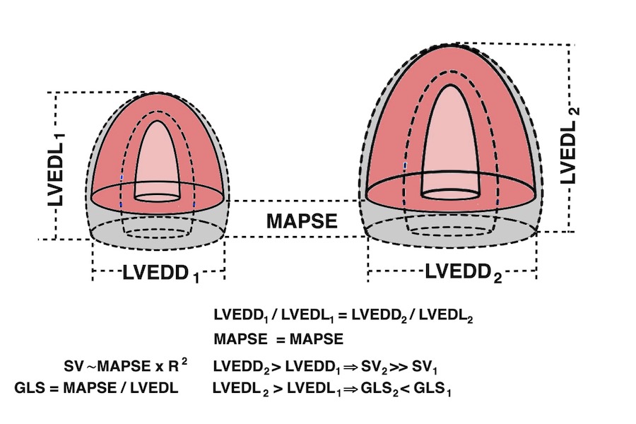
Relation between systolic longitudinal ventricular shortening / MAPSE and stroke volume
The eggshell model of the heart would predict that the stroke volume would be solely the function of long axis shortening (12 - 14), at least with an incompressible myocardium. As discussed in the basics section, however, there is an outer diameter decrease as well (62, 63, 65), contributing to stroke volume. With a completely incompressible myocardium, the stroke volume would equal the reduction in outer volume, without taking cavity and wall thicknesses into consideration. As the incompressible myocardial volume remains constant, the outer volume reduction must equal cavity volume reduction as shown below.
The left figure shows the cavity volume reduction, being the function of longitudinal and endocardial transverse diameter shortening. But the right figure shows that the total LV outer volume is the sum of cavity and myocardial volume. Given a minimally incompressible myocardium, the reduction in total volume = reduction in cavity volume, while the myocardial volume is constant.
Total (outer) LV volume LVTV = Cavity volume + myocardial volume (MV).
Diastole: LVEDV = LVEDTV - LVEDMV
Systole: LVESV = LVESTV - LVESMV
SV = LVEDV - LVESV = (LVEDTV - LVEDMV) - (LVESTV - LVESMV) = LVEDTV - LVEDMV - LVESTV + LVESMV
If the myocardium is nearly incompressible is LVEDMV
Stroke volume
Outer volume decrease has two components:
Longitudinal component = MAPSE × Mitral annular outer area = MAPSE ×
Transverse component which is SV - longitudinal component.
In the HUNT study we used a symmetric, ellipsoid model of the LV, In the HUNT3 ellipsoid LV model, (65), we measured MAPSE and outer ventricular diastolic and systolic diameter, and assumed the mitral annular diameter to be equal to LV outer systolic diameter as shown by the figure above. Thus we calculatedThe SV from the cavity volumes, MAPSE × mitral annular area, to derive the MAPSE part of the SV, considering the remaining decrease to be due to the ourer LV diameter decrease. We found that MAPSE contributed 74.2% of total SV. Circumferential shortening due to OUTER circ. (diameter) shortening, was 12.8%, and must make up the rest, 25.8% of SV.

Although all primary measurements were normally distributed, the volumes were not, indicating that there was a systematic error in the geometrical model. This is reasonable, as the assumption of the model was a symmetric ellipsoid, which is not the case in real life.
In this model, the correlation between MAPSE with SV was still only 0.25, and with EF 0.16 (both P < 0.001). This is the inter personal variability.
 |
 |
| MAPSE
vs SV, shows a modest
correlation, due to both
variability of measurements,
the variability due to age and
to the contribution of the
cross sectional contraction
(outer FS/circumferential
strain. |
MAPSE
vs EF, showing an even more
modest correlation. |
Direct measurement by MR have shown that the AV-plane contribution is closer to 60% for the LV, but ca 80% for the RV (66, 67,68), which probably is closer, although a study of LV filling found that systole contributed 70% to ventricular filling, which should be equal to the ejected volume unless there is concomitant atrial expansion also.
In the HUNT3 study, using the ellipsoid model, Global MAPSE correlated woth normalised global MAPSE (R=0.86), GLS by segmental strain (R=0.40), S' (R=0.34), SV (R=0.25) and EF (R=0.16), all p<0.001). The two methods for GL correlated with each other (R=0.52), with S' (R=0.26 and 0.44, respectively), with EF (R=0.22 and 0.24), all p<=.001).
Longitudinal
strain / Relative shortening
Thus, as discussed above, in this text
longitudinal strain is considered as
"relative shortening",
Relative
shortening (Longitudinal systolic
strain) is basically MAPSE normalised
for LV length
Longitudinal systolic strain and MAPSE are related, as longitudinal strain basically is MAPSE normalised for LV length (18). It does seem intuitive that normalising MAPSE for length (ventricular or wall), should reduce the part of biological variability due to body size (heart size). In the HUNT study, however, we found that both segmental strain by tissue Doppler (17), as well as by the linear method (MAPSE normalised for wall length) (18), had similar relative standard deviations as non-normalised MAPSE. The finding that normalisation for LV length did not reduce biological variability, was perhaps a bit surprising, but is explainable as age is the source of the most variability (18)
However, while there was a positive correlation between MAPSE and BSA, which was weak, however, only 0.12, we found stronger, but negative correlations between both tissue Doppler derived GLS, and normalised MAPSE, of -0.23 and -0.27, respectively. This seems to indicate that the normalisation itself, induces this, which seems like a systematic error.

Relations of MAPSE, MAPSEn, and GLS to BSA. The figure shows a weak tendency of MAPSE to increase with increasing BSA, although the tendency is slight, and not enough to induce gender difference.
MAPSE was not significantly sex dependent (although with a trend of 0.1), while both GLS and normalised MAPSE were significantly higher in women (p=0.001), but by linear regression only BSA remained significant, so the sex differences are an effect of differences in size between sexes (18).
But what is the explanation of this apparently counterintuitive finding?
It is due to the fact that both LV length and diameter are related to BSA, and they are proportional (19). As the greater part of the SV is related to MAPSE × cross sectional annular outer area (radius squared), and as a larger ventricle has a larger cross sectional annular outer area, there can be a larger SV with the same MAPSE, so the adjustment of SV for a larger body and heart, do not necessitate an increase in MAPSE. But as the larger ventricle is longer, the strain denominator is bigger, and the absolute value of strain is lower, despite the unchanged MAPSE.
MAPSE correlates with SV and EF, GLS
do not correlate with SV, only with EF
Despite the fact that MAPSE correlates
with SV, Global strain does not, and as
this is by either method, so the effect
seems to be systematic. Global strain on
the other hand, correlates with EF (156),
as also shown (109)
in experimental studies of intraperson
(-animal) variability. In inter personal
variability, the relation of MAPSE and
global longitudinal strain depends
on the method for GLS, and We found
a correlation of MAPSE with linear
strain (MAPSE normalised for linear
wall length) of 0.86 - not surprisingly,
but with Global
segmental strain of 0.40.In the HUNT3 study, using the geometrical model, Global MAPSE correlated with normalised global MAPSE (R = 0.86), GLS by segmental strain (R = 0.40), S' (R = 0.34), SV (R=0.25) and EF (R = 0.16), all p < 0.001). The two methods for GLS correlated with each other (R = 0.52), with S' (R = 0.26 and 0.44, respectively), with EF (R = 0.22 and 0.24), all p < 0.001). However, GLS by either method do not correlate with SV (156). The possible explanation is the previous finding that SV is related to both LV length and diameter, which are interrelated, while global LV strain only normalizes for LV length, thus introducing a systematic error as described above. The SV in this comparison, however, is derived from a geometrical model (65), which in itself may include a systematic error, but the concordant results between the two strain methods, as well as the maintained relation of SV with MAPSE and S’, supports this finding.
As SV and MAPSE increases with BSA, and GLS decreases with BSA, this lack of correlation was not surprising.

Diagrams, showing that MAPSE corelates with both EF and SV, while GLS by boith methods only correlates with EF, not BSA.
The reason for this is the relations to BSA, as explained above.
While global strain is related to EF, as seen below,

the volume changes of ejection and filling are closely related to the changes of the LV longitudinal dimension
Longitudinal strain
measurement depends on method, and there is no gold
standard for global longitudinal systolic strain
Linear strain
If we just consider a simple Lagrangian measurement of systolic longitudinal strain this should be fairly simple, being LV systolic shortening / LV end diastolic length:
 |
 |
|
Lagrangian
strain is the relative shortening
normalised for the end diastolic length. LV
shortening = diastolic - systolic length,
|
LV shortening can also be measured by M-mode as the mean MAPSE, the relative shortening is then the normalised MAPSE = MAPSE / Ld. |


As we see, end diastolic LV length < end diastolic WL by straight line from mitral ring to apex, which again is < by the curved length along the wall, and the numerical value of the strain decreases with the increasing denominator. We used the straight line WL approach in the HUNT study (7, 18), for better reproducibility, as the data quality was less, and automated edge detection was not so good. This method is robust and reproducible, and represents what we can call linear strain (by linear measurements). Mean diastolic WL was 9.47 cm, and mean strain by MAPSE / WL (calculated per subject an wall an then averaged, was -16/3% (SD=2.4).
A smaller study using the same method, found similar strains in the healthy control subjects (24) as in the HUNT. Longitudinal strain by direct manual measurement of longitudinal dimensions, have also been used in MR (25), but here the mid ventricular long axis was used as denominator. This study demonstrated that even the small variations in end diastolic length using mid ventricular versus a 90° axis on the mitral plane resulted in slightly different longitudinal strains. The choice of epicardial versus endocardial end point, of course affected both numerator and denominators, so here, the difference was bigger. All in all, means for healthy volunteers varying from -15.9 to -21.1%.
Thus, again the absolute value of strain is dependent on the choice of denominator, as illustrated by the following example:

For any given MAPSE, the global strain will be determined by the choice of denominator. In this case, mean MAPSE is 1.7 cm. End diastolic length will be the denominator in the strain equation. Using the mid ventricular line (blue), gives the smallest denominator and thus the highest global strain value of 17.3% in this example. Using wall length, will result in a higher denominator, resulting in lower GLS value, the straight line approximation (green) gives an intermediate denominator and a GLS value in this example of 16.3%, while the curved lines (red) following the walls gives the highest denominator, and thus the lowest GLS value, in this example 14%.
Wall strain vs LV strain:
Using an ellipsoid model of the LV, calculated mean LV
mid cavity length was 92.4 mm external, and 88.8 mm
internal length. Mean MAPSE was 15.8 mm, which would
result in a relative LV shortening
(as opposed to wall shortening) of 17.1% using the
external diameter, and 17.9% using internal diameter.
This shows the effect of choosing the denominator.

The true numerator in the longitudinal strain,
Segmental strain and strain rate:
It is customary to divide each wall into three segments,
corresponding to basal, midwall and apical levels. This
results in 18 segments, and for evaluation of regional
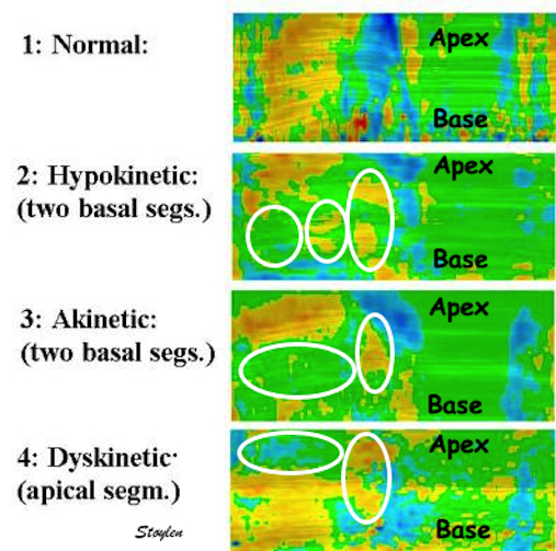
function, this 18-segment division works well. The regional systolic function is traditionally shown as wall motion score:
- Normal
- hypokinetic
- Akinetic
- Dyskinetic
 |
 |
I |
| Segmental division of the left ventricle. The segments are related to different vascular territories, as shown by the colours. However, in the figure given in that paper, the apicolateral segment is given as Cx or LAD, while the apical inferolateral is not, despite the model is only giving four segments in the apex. Thus, there is a slight inconsistency. | n WMS = 2, there is both hypokinesia and tardokinesia as well as PSS, in WMS 3 there is PSS and in WMS=4, there is dyskinesia and PSS in the apical segment, but also PSS inthe midwall segment indicating a more extensive partial ischemia. |
Regional function can thus be evaluated by WMS, Segmental longitudinal strain rate or segmental longitudinal strain.
 |
 |
 |
| Segmental strain by
speckle tracking |
Longitudinal strain curves and peak systolic values from the recording to the left. | Segmental strain by tissue Doppler from the HUNT study. |
Segmental evaluation is possible by all strain modalities.
Speckletrackling
 |
 |
However, when segmental strain is averaged to global strain, the varying amount of myocardium in the different levels may matter. Basal and midwall levels have more myocardium, the apex less, as it is both thinner and has a smaller circumference.
Thus the original ASE segmental model had 16 segments (244), where the apical lataral and inferolateral, and the apical septal and anteroseptal segments were averaged, giving four apical segments instead of six. (It may also have been a matter of convenience, as it was customary to acquire only apical 2ch and 4ch images, and parasternal long axis image, so only four segments were available. Newer guidelines allows more lenience (224).
The HUNT4 study, comparing the 16 and 18 segment model (245) found significant, although minimal differences between different applications (although all by speckle tracking, and from one vendor) and segmental models.
Segmental strain and strain rate by tissue Doppler in the HUNT3 study:
In the HUNT study, the original automated method was based on placing kernels at the segmental borders, tracking the motion of the kernels through the heart cycle (17).
 |
 |
|
| Serch areas for
kernel tracking from frame to frame, oraqnge,
lo0ngitudinal search areas by tissue Doppler,
white areas transverse serch areas for speckle
tracking. |
Segmental strain by tracking
kernels at the segmental borders, either
calculating strain from segment length, or using
the segments for placing the ROI for the velocity
gradient. |
Real time tracking
of kernels at the segment borders. |
The method was supposed to track longitudinally by tissue Doppler, and laterally by speckle tracking.
|
 |
 |
| Real time tracking of kernels at the segment borders. | Strain rate curves.
Green: average of three segments of the wall,
blue, curve for each segment |
Strain curves. Green: average of three segments of the wall, blue, curve for each segment |
Basically this could lead to three different methods.
- Automated segmentation, and tracking the kernels,
calculating (Lagrangian)
strain and deriving (Eulerian)
strain rate.
- Automated segmentation, placing the ROI for the velocity gradient at the segmental middle. This would be similar to the commercial method using stationary ROIs.
- Automated segmentation, but tracking the kernels, and letting the ROI follow the segmental middle.
Method 1 was the method applied to the total material of 1266 giving a mean peak strain rate of - 1.03 s-1 (SD = 0.13) and mean end systolic strain of - 16.7% (SD = 2.04) (17). For strain, this is fairly similar to the linear strain we found in the re analysis (7, 18) by simply measuring the MAPSE normalised by the (straight line approximation to) wall length as shown above, which gave a mean strain in the total material of -16.3% (SD = 2.4).
As both of these gives lower values than speckle tracking methods, which possibly is due to speckle tracking following both longitudinal and inwards motion as discussed below, while the velocity gradient derived strain is fairly similar, it seems that this segmental method mainly did longitudinal tracking of the kernels, and the segment lengths were the result of this longitudinal tracking by tissue Doppler, while transverse tracking by speckle was negligible. The reasons for this, is probably:
- Kernels were placed in the middle of the wall, where inward motion is less than in the endocardium.
- Tracking was done in the tissue Doppler loops, where the B-mode frame rate was low, which also means that there was a low lateral resolution for tracking.
Comparing with the velocity gradients obtained by the automatic segmentation in a subset of 57, we found peak strain rate of -1.45 (0.79) s-1 and strain of -17.7 (8.5)% by the stationary ROI (method 2) and -1.43 (0.67) s-1 and -16.7 (8.1)% respectively by the tracked ROI (method 3). This compared to -1.08 (0.25) s-1 and 17.4 (3.4)% by method 1 in the same subset. Obviously, peak strain rate values are far higher numerically by velocity gradient than by segment length, while strain values are similar. This is due to the high noise content of the strain rate, which affects the peak values. As strain rate is the difference between velocities (the spatial derivative), while the noise is the sum of the relative errors of the velocity measurements, the signal-to-noise ratio is far less favorable in strain rate imaging than in velocity imaging.
 |
 |
| A
moderately noisy (unsmoothed) velocity signal. |
Unsmoothed
strain rate curves from the same loop and
segments. The increase in noise by the spatial
derivation is evident. |
Random noise in strain rate
Noise in
strain rate , and thus peak values are affected by both
strain length, ROI size and temporal smoothing:
Effect of temporal smoothing and strain length
Integration of strain rate to strain, will eliminate random noise as well, even without any other smoothing as shown below:
|
 |
| Noisy
(unsmoothed) strain rate curve. |
Strain
from the same loop and segments. No specific
smoothing has been applied, but the intergration
itself eliminates the random noise |
Global strain and strain rate is obtained by measuring in each se3gment, and taking the mean, but excluding segments with obvious artefacts.
Strain rate by velocity gradient is a noisy method, where peak values are very much dependent on noise and thus the amount of temporal and spatial smoothing applied, as well as strain length. However, strain is less affected by random noise, so all three methods give comparable strain values, but still will be influenced by both frame rate and beam width, as well as insonation angle. Tissue Doppler is limited to tracking in the direction of the ultrasound beam, and is thus vulnerable to angle distortion,
Feature tracking results in higher
absolute strain values due to simultaneous inward tracking
The term
"tissue tracking" was used for the integration of tissue
velocities into displacement, but based on colour tissue
Doppler (26). But as this was an
indirect method of deriving tissue dispolacement, methods
using direct tracking of tisssue markers, is called feature
tracking (mostly used in CMR, and which can be applied
to ordinary cine MR(27)), or speckle
tracking (mostly used in ultrasound, and which can be
applied to ordinary B-mode echocardiopgraphy (28)).
The tracking is based on the recognition of patterns of features or irregularities in the image to be recognised as a pattern, and following them in the successive images of a sequence. In echocardiography ventricular myocardium typically shows a speckled appearance that is relatively stable through parts of the heart cycle. The details of the speckle tracking method will be described later. In general, the feature tracking methods begins by identifying a window (kernel) in one image and searching for the most comparable pattern in a window of the same size in the subsequent frame. The displacement found between the two patterns is taken as the local displacement of the tissue, and the differential motion will be the deformation:
 |
 |
 |
| Following the kernel through a whole heart cycle, will lead to a displacement curve shown to the right. Temporal derivation (displacement per time, or frame by frame displacement divided by the time between frames) results in the derived velocity curve shown below. |
From two different kernels, the
relative displacement and hence, strain as well as
strain rate can be derived. The strain obtained by
simply subtracting the two displacements and
dividing by the end diastolic distance is the Lagrangian strain. To obtain the Eulerian
strain rate, the correction has to be applied for
each frame. |
If Kernels are placed at the segmental borders, the result will be segmental strain and strain rate in six segments per plane. |
 |
|
| Longitudinal speckle tracking in apical 4 chamber view. Tracking of inter segmental kernels shown in motion. | Speckle tracking can be applied crosswise. In this parasternal long axis view, the myocardial motion is tracked both in axial and transverse (longitudinal) direction. It is evident that the tracking is far poorer in the inferior wall, due to the poor lateral resolution at greater depth. |
With a greater number of kernels, distributed both along and across the wall, each kernel can be tracked individually, and displacement and velocity can be measured in two dimensions, both longitudinally and transversally for each (29).
 |
 |
 |
|
Visualisation of speckle tracking.
Here, the midline of the ROI is tracked for
longitudinal strain. The bullets seem to follow
tissue motion, but the may well be due to the
algorithms rather than the tracking. |
Speckle tracking
where trackin is done in both longitudinal and
transverse direction, Thus, in principle, both
transmural and longitudinal strains are available,
depending on the lateral resolution in the imag
(which generally is poor in the basal parts. |
Longitudinal strain curves and peak systolic
values from the recording to the left. |
Feature tracking has to be optimized, with adjustments for image quality, temporal resolution, speed and magnitude of the expected displacements. In addition, there has to be smoothing for random noise, basic technical underlying algorithms for tracking such as choice of kernel sizes, selection and weighting of acoustic markers, stability of speckles, and drift compensation during heart cycle, as well as spatial smoothing along the ROI. Finally, the ROI shape itself has effect.
A joint EACVI/ASE/Industry Task Force has attempted to standardise measurements across different echo platforms (6),
for:
- Segmentation
- Measurement points
- nomenclature,
As with all other strains, speckle tracking strains rest on assumptions: , width of the ROI, In addition, the black box ST applications all have complex algorithms with
different choices for
-Assumptions of LV shape and ROI width
-Mid/mean vs endocardial
-Number, size and stability of speckles
-Weightinhg of speckles
-Decorrelation detection and correction
-Spline smoothing along the ROI and weighting of the AV -plane motion
-and especially relation between apical and basal width, weighting and numbers of apical segments, as the curvature is biggest in the apex.
-etc.
 |
 |
| Speckle tracking
image of the LV. The tracking bullets at the outer
layer move least inwards in systole, the bullets
at the endocardium move most, the mioddle row
intermediate. Thus, there is a gradient of inward
motion across the walls. |
This is shown
diagrammatically. End diastolic outer contours in
unbroken lines, end systolic contours in broke
lines. Outer contour (black) moves least, inner
contour (blue) moves most, midwall contour (red)
intermediate. |
Looking at the images above, it is evident that there is a gradient of inward motion from the epicardium to the endocardium. This is due to geometric factors (not fibre or layer function), and will be present in all methods using crosswise tracking. This inward tracking, however, will result in apparent longitudinal shortening of the midwall and endocardium, even, hypothetically, without any ventricular shortening at all. This is due to the conical shape of the LV:

Hypothetical wall thickening, even without wall shortening. As the wall thickens, both the midwall (red unbroken) and the endocardial (blue unbroken) end diastolic lines move inwards. This is true for both the curved lines and the straight lines, the dotted lines (end systole) being shorter than the unbroken lines (end diastole). The inward motion shortens the lines, leading to a measurable longitudinal wall strain, even without any shortening of the LV.
In real life, there is simultaneous wall shortening and thickening. The additional longitudinal strain is thus a function of wall thickening, but the thickening is mostly a function of shortening.

Simultaneous wall shortening and thickening. As the wall shortens, it has to thicken, due to conservation of the myocardial volume. As illustrated above, the mid and endocardial lines shorten not only due to wall shortening, there is a shortening due to the inward movement as well, which again is caused by wall thickening. And as wall thickening is due to wall shortening, this means that the shortening is speckle tracking strain is over estimating the true wall shortening.
This wall shortening due to the inward motion, is thus an artefact, due to inward tracking, and may be the most important reason why the normal values for speckle tracking derived strain lies higher in absolute values, compared to linear strain. Mean global longitudinal strain in larger normal studies with speckle tracking is -19 to -21% (38 - 41), and very similar in in CMR feature tracking (31).
Although a direct comparison is not done, the HUNT3 study used segmental linear tissue Doppler derived strain and linear strain , and found mean longitudinal strains of -16.7% and -16.3%, respectively.
In the HUNT4, this was evident. In the same population, long axis dimensions were measured, and GLS by speckle tracking in the same population, showing even lower vavlues for relative shortening by direct measurement, than by speckle tracking:
Comparing with the values from HUNT4 (245, 249), which were measured in 2D the values according to age and sex can be found in the original publications.:
| Age (Years) |
LVLd |
LVLs |
Syst. shortening |
Rel. shortening |
| Women | ||||
| 20 - 39 |
8.5 |
7.2 |
1.3 |
0.15 |
| 40 - 59 |
8.3 |
7.1 |
1.2 |
0.14 |
| 60 - 79 |
7.9 |
6.8 |
1.1 |
0.14 |
| > 79 |
7.1 |
6.4 |
0.7 |
0.1 |
| All |
8.1 |
7.0 |
1.2 |
0.14 |
| Men | ||||
| 20 - 39 |
9.7 |
8.1 |
1.6 |
0.16 |
| 40 - 59 |
9.2 |
7.9 |
1.3 |
0.14 |
| 60 - 79 |
8.9 |
7.7 |
1.2 |
0.13 |
| > 79 |
8.5 |
7.2 |
1.3 |
0.15 |
| All | 9.1 |
7.8 |
1.3 |
0.14 |
| Total |
8.5 |
7.3 |
1.2 |
0.14 |
19.8
GLS is by speckle tracking, from (245), which is the same population (for comparison with absolute and relative shortening, GLS is given by numerical values):
| <40 years |
40 - 49 years |
50 - 59 years |
60 - 69 years |
> 69 years |
All |
| Women |
|||||
| 21.3 |
21.0 |
20.5 |
19.7 |
19.0 |
20.2 |
| Men |
|||||
| 19.8 |
20.1 |
19.5 |
18.9 |
18.5 |
19.3 |
| Total: 19.8 | |||||
As predicted, the HUNT4 (245), using GE hardware and speckle tracking analysis software, found mean GLS of -20%, but even within the domain of speckle tracking, the NORRE study (39), using a mix of GE and Philips hardware, and TomTech analysis software foun mean of -22.5%.
It may seem that LV strain is closer to the values by speckle tracking, but the values are achieved by different means, speckle tracling by measuring wall shortening, due to longitudinal shortening plus shortening effect of inward tracking, while LV shortening as opposed to wall shortening is due to shortening of the mid cavity length, being less.
Longitudinal layer strain is an artefact from inward feature tracking.
In the Argument above, it is shown that there is a gradient
of inward tracking from the outer to the inner contour of
the wall. This inward tracking will thus in itself cause
shortening, which is due to geometry, and comes in addition
to the longitudinal shortening of the wall. But as there is
a gradient of inward motion, there will also be a gradient
of shortening across the wall. This is easily demonstrated
by speckle tracking,

Speckle tracking where longitudinal strain is measured in three different layers, showing the absolute values to be greatest in the endocardial layer (23.5%), smallest in the outer layer (17.4%) and intermediate (20.2%) in the midwall layer which is taken as the global strain.

Illustration of the torsion of the mitral ring that would result if the longitudinal layer strain had true longitudinal shortening ain addition to the effect of inward movement.
CMR feature tracking has shown the same phenomenon, higher absolute values in mean systolic global endocardial longitudinal strain than mean global (mid) myocardial longitudinal strain; 19.2 ± 3.6% vs 21.0 ± 3.9% (31). This seems to confirm that CMR feature tracking shows the same effect of inward tracking asn ultrasound speckle trackibng, and that the global values are a combination of inward and longitudinal deformation.
Both transmural and circumferential strains must be measured in short axis views. In principle, transmural strain could be measured in apical views, but at least for ultrasound speckle tracking, but the decreasing lateral resolution with depth precludes transmural measurements from apical images in the base. In fact, that option was removed after we pointed it out.

Transmural strain
Transmural strain is also called
"radial strain", which means "in the direction of
the ventricular radius". However, in ultrasound
terminology, the "radial direction" is also used
synonymously with "in the direction of then
ultrasound beam", so the term is ambiguous.Transmural strain is simply relative wall thickening. There is no such thing as "transmural myocardial function", as there are no transmural fibres. Wall thickening is mainly due to longitudinal wall shortening, it must thicken in the transverse direction to conserve myocardial volume partially or completely.
When the ventricle shortens, the wall will thicken. Wall thickening is transmural strain (thickness increases; i.e positive strain).
 |
 |
| Deformation in systole.
Left: end diastolic image, showing the
end diastolic length (Ld =
L0). During systole, the
ventricle shortens with |
Wall thickening. Systolic wall thickening equals systolic transmural strain |
Wall thickening can be measured by simple caliper measurements of wall thickness in systole and diastole as percentage wall thickening (positive strain: thicker in end systole).
WT = (WS - WD)/WD =
 |
 |
|
Transmural strain by M-mode. The
M-mode measurement is more accurate than 2D
measurements, but are only feasible in the septum
and inferolateral (posterior) wall. |
The average of septal and inferolateral wall should be used, as septal thickening is less than inferiolateral wall thickening. |
Mean transmural strain by this method in the HUNT study was 56.5 (SD:19.6)%, which is in accordance with older findings with M-mode (32 - 35), B-mode (36) and MR tagging and ultrasonomicrography (37).
Transmural strain can be measured by speckle tracking as shown below. It has to be measured from short axis images, as the decreasing lateral resolution with depth precludes transmural measurements from apical images. In fact, that option was removed after we pointed it out. However, the speckle tracking method enables measurement of transmural strain in all segments across the wall.
 |
 |
| Speckle tracking in short axis cine loop | Resulting peak strain values and strain curves from the tracking. |
Multi centre studies of speckle tracking derived strain, however, have shown rather wildly varying normal values from 37.4 to 88% (38 - 41), with most studies showing lower values, and the same for CMR feature tracking 34.5± (31). Basically, transmural strain should be in accordance with known wall thickening.
There is no such thing as transmural function. Transmural strain is thus in itself not a function measure. This is hardly surprising, as there are no transmurally directed fibres. Wall thickening reflects the thickening of the individual muscle fibers inn all directions as they shorten and are displaced inwards as discussed below. Transmural strain is a measure of deformation, not of function. It is simply a component of the strain tensor, or a coordinate of the total three-dimensional deformation.
Longitudinal shortening will lead to wall thickening. This would have been true, even if there had been only longitudinal fibres.
Gradient of
transmural strain.
As
discussed above, wall thickening is mainly due to wall
shortening and conservation of volume. Considering wall
thickening separately,mthis alone will explain the gradient.
The systolic thickening occurs inward, as the outer contour
of the LV decreases in systole as discussed below. The fact
that the wall thickens inward, means that the myocardium
moces from an area of larger to smaller circumference, and
thus, to conserve volume has to thicken concordantly. This in itself induces a gradient of thickening from the outer to the inner contour, which was described as early as 1991 (42, 43). Since there is no radial function, this gradient is of course not related to differential fibre function, but is simply a geometric effect.
If we consider the thickening due to wall shortening first, it is useful to consider the wall as two layers as shown below. The thickening of the outer layer (due to longitudinal shortening) will push the inner layer inwards. The inner layer than has to thicken due to there being less room in the inner part of the cavity. In addition, the inner layer shortens as well, and will thicken due to the conservation of the volume, so the inner layer has to thicken even more than the outer.
Gradient of thickening illustrated by two layers: Left, end diastole. Disregarding outer contour decrease, the outer layer thickens due to longitudinal shortening (middle). That means the outer layer pushes the inner layer towards the centre, where there is less room. This effect alone will cause the inner layer to thicken due to the reduced diameter. In addition, the inner layer also shortens due to longitudinal shortening. This means that the inner layer thickens due to both shortening and inward displacement, and thus thickening more than the outer layer.
In addition there is a component of outer diameter (and circumferential) shortening (7), which will contribute to inward displacement of all layers of the wall, and thus to the total wall thickening:
In addition, there is systolic outer diameter / circumference decrease, due to circumferential fibre shortening. In fact, the outer diameter circumference shortening is the true circumferential fibre function, as will be shown below. Circumferential shortening will lead to a modest reduction in outer diameter, and circumferential shortening. Basically, this means that the outer diameter shortening also is a contributor to wall thickening, pushing all wall layers inwards, and the amount of wall thickening is also related to outer circumferential shortening.


Thus:
- Outer circumferential shortening, displaces the whole wall inwards, contributing to thickening.
- Longitudinal shortening of outer layer causes more thickening of outer layer and displaces inner layer further inwards.
- More inwards displacement of inner later causing more thickening of this layer due to inwards displacement
Circumferential strain
The main facts of LV circumferential strains are:- Circumferential strain can be measured by speckle tracking, but also by diameter measurements, being equal to diameter shortening.
- 131, There is a gradient of circumferential strain from
outer to inner surface.
- Only outer circumferential strain is a function of
circumferential fibre shortening, both the midwall and
endocardial circumferential strains as well as the
gradient are mainly a function of wall thickening.
1: Circumferential
strain equals diameter shortening
Circumferential strain means systolic shortening of a circumference, which then is negative strain:
But as fractional shortening is FS = (DD - DS) / DD,

As diameter and circumference are proportional, fractional circumferential shortening and diameter shortening are equal.
2: There is a gradient of transmural strain from the inner to the outer surface.
This was described already 1991 by MR tagging , and later by Echocardiographic speckle tracking (42). The interpretation, however, was that this was due to differential function of the different layers. However, the fact that midwall fractional shortening is less than endocardial, is also well known (43), and from the above discussion, the

In the HUNT study (7), Endocardial diameter was measured directly, and outer diameter (LVED) was calculated as LVED=LVID+IVS+LVPW both in diastole (LVEDd) and systole (LVEDs). Endocardial and external fractional shortening (FS) was calculated from internal and external diameters in diastole and systole in the ordinary way. Midwall FS was calculated from LVID + (2×1/2 WT) in systole and diastole, respectively.
The circumferential strains were:
| Endo-card εC | Midwall εC | External εC |
| -36.1 (7.3) |
-22.7 (4.9) |
-12.8 (4.0) |
It is important to realise that MR tagging tracks actual points in the myocardium, meaning that the systolic midwall circumference conforms to the midwall in diastole, while the midwall FS /
The gradient of circumferential strain is also seen with speckle tracking.

Circumferential peak systolic layer strains, varying from - 32.4% in the endocardial layer via -17.3% in the midwall layer to - 6.9 in the outer layer.
In speckle tracking, the principle is tracking of material points, but due to the averaging functions, the midwall line seems to stay in the geometric wall middle.
3: Only outer circumferential strain is a function of circumferential fibre shortening, both the midwall and endocardial circumferential strains as well as the gradient are mainly a function of wall thickening.
The finding of the gradient of circumferential strain, has been interpreted as differential circumferential fibre function (shortening). However, this is faulty. In a thickening wall, both midwall and endocardial circumferences will move inward simply because of inward thickening. And as there is a gradient of wall thickening, there will be a gradient of circumferential strain as well.

Outer circumferential or diameter shortening is due to circumferential fibre shortening, no other mechanism is conceivable.
- Outer
circumferential shortening displaces the wall inwards,
and is part of the total circumferential strain.
- Outer layer thickens due to both inward displacement and longitudinal shortening, and this displaces midwall circumference more inwards.
- Inner layer thickens more, both due to inwards displacement from outer circumferential shortening and from outer layer thickening, and inner layer thickens even more due to inner layer shortening, displacing the endoocardial surface even more inwards.
Actually, the fact that the inner layer thickens
into a much less space, means it has tho thicken more. But
this also means that the midwall circumference moves
inward also in relation to the tissue itself, and does not
relate to then mid line of the tissue. Thus:
- The outer circumferential strain reflects circumferential fibre shortening
- Midwall circumferential
strain is the most representative, and the one
demonstrating the interaction between strains, but is
partly a function of wall thickening, which again is a
function of
- longitudinal shortening and
- circumferential outer shortening and wall thickening
- Endocardial
circumferential strain equals fractional diameter
shortening, but is mainly wall thickening
 |
 |
| Circumferential
strain calculated from a hypothetical,
symmetric, half ellipsoid model with a diastolic
mid wall thickness of 0.9 mm (decreasing towards
apex), an outer diastolic diameter of 60 mm, a
diastolic length of 95 mm. Wall thickening is
calculated from longitudinal shortening and
conservation of wall volume, given different
outer circumferential strain or shortening. Wall thickening is calculated from longitudinal shortening and conservation of wall volume, given different degrees of outer contour change (outer circumferential strain or shortening). |
|
| Midwall and endocardial circumferential strain as functions of wall thickening, for 0%, 5% and 10% outer diameter reduction. | As wall thickening also is a function of longitudinal strain, midwall and endocardial strain as functions of longitudinal strain, for 0%, 5% and 10% outer diameter reduction. |
Linear strains derived from B-mode in the HUNT study are summarised:

Linear strains in three dimensions. Longitudinal shortening. Longitudinal strain can be measured by systolic and diastolic left ventricle (LV) lengths (A) or by Annular motion (B) divided by wall lengths (A). Transmural strain to be a truly segmental measure (C), the quantitative equivalent of wall motion score. The circumferential strains can be seen to be related to outer circumferential shortening as well as wall thickening, and endocardial circumference can be seen to move most, external most. As circumferences can be calculated from diameters, circumferential strains can be calculated from fractional shortening. Midwall and external circumferential strains were calculated from endocardial diameters and wall thicknesses.
The interdependence between strains can be summarised in the following figure:

Thus, the principal strains are governed by geometric relations, not fibre directions. Given the strong interrelation between strains, most of the information about global systolic deformation can be gleaned from the longitudinal strain.
Area strain
Hypothetically, composite measures might contain more information, integrating information in more than one direction. However, as area strain is not part of the original Lagangian definition, the concept needs a definition, one reasonable candidate is simply the systolic relative reduction in area, giving an analogous definition to the one concerning one dimensional strain:
 |
 |
 |
 |
 |
 |
| Area strain. As the ventricle contract, the end diastolic area of the selected region (red) would be reduced in both the longitudinal and circumferential direction. Assuming a cylindrical shape of the segment, the area will be equivalent to a flat geometry. In the apex, the shape would be more triangular, which means the area is only half that. Both the cylinder and triangle will underestimate the true area, as the surface is curved, but the underestimation will be similar in end systole and end diastole, so the area strain approximation will be closer to the real area strain. | Area strain is a function of longitudinal strain. |
One dimensional strain is defined as
L - L0 =
L =
Thus:
A = L0 (
And:
Thus area strain is

Regional
strain and strain rate
Regional
segmental strain also reflects segment interaction.
Segmental strain do not only reflect segmental
contractility, but also interaction with other
segments.Both differences in onset of tension, different tension during contraction and differences in timing will give segmental inequalities in shortening.Simultaneous shortening of one part of the ventricle and and stretching of another, occurs when there is tension imbalance.
This may occur physiologically during the IVR (72), and in regional dysfunction, mainly in regional ischemia as discussed below, and in conduction disturbances
Segmental dysfunction results in reduced shortening. This is usually due to ischemic heart disease, and may result from
- Acute ischemia
- Stunning
- Hibernation
- Necrosis
- Necrosis with scarring
 |
 |
|
Segmental division of
the left ventricle. The segments are related to
different vascular territories, as shown by the
colours. As
we see, all walls (except the anterior
free wall) belongs to more than one vascular
territory. |
Top: segmental shortening of the septum,
left :strain rate, right: strain. Bottom, the
resulting motion of the segmental borders,
where the apical shortening pulls the midwall
and basal segments along, imparting motion,
and the midwall segmental shortening imparts
an additional motion to the basal segments.
Left velocities, right displacement. |
This causes
- The affected segments to shorten less
 |
 |
This can also be recognised by the separation of the velocity or displacement curves.

Left: Normal ventricle, right: small apical infarct, top: strain rate, below: velocity curves. In the normal ventricle, the systolic strain rate can be seen to be relatively similar in all three segments, about - 0.9 s-1. This corresponds to a relatively even spacing of the velocity curves. In the infarcted ventricle the apical segment can be seen to have strain rate of about - 0.5 s-1, compared to the normal strain rate of -1s-1 in the midwall and basal segments. Looking at the velocity curves below, the two points bordering the apical segment (red and green) can be seen to be very close to each other, indicating that they move as a stiff piece without deformation.
Just inspecting the velocity curves is thus a way of visualising the strain rate without measuring it.
Segmental strain
with other segments interact through both contractility
and load.
In addition:
- Neighboring unaffected segments shorten more due to
reduced segmental load,
as not only shortening, but also tension is reduced in
the affected segments.
- Global left ventricular shortening to decrease in
proportion to the amount and extent of the total
segmental reduction in contractility.

Segmental interaction in a two level model of the LV. To the left a normal ventricle with equal tension and shortening in all segments, resulting in homogeneous shortening (orange colour), and an ordered gradient of motion from the base, decreasing tom the apex (fat arrows). Middle, reduced tension in the right base (shorter arrows), resulting in reduced shortening (yellow colour). As the tension in the basal segment is reduced, this results in increased shortening of the neighboring apical segment (red colour), despite normal tension (unchanged arrow length) as the segment contracts with less load. But as the total contractility of the ventricle is reduced, due to the segmental hypofunction, the total LV shortening is reduced (fat arrow in the base). Right, reduced tension in the right apex, in this case, as the apex is not anchored the same way, resulting in apical stretch (blue colour). The low tension in the apex, again results in increased shortening of the base (red colour) with unchanged tension, due to reduced local load.
We did show this combination of hypokinesia in infarcted segments, together with hyperkinesia in non-infarcted segments. In addition, as part of the acute dysfunction in infarcts is stunning that can reverse with successful reperfusion, the accompanying hyperkinesia reversed simultaneously with the recovery of stunning (92).
Regional MAPSE
cannot identify infarct site, only infarct size
This mechanism may be part of the reason why the mitral ring motion is universally reduced around the circumference, and not specifically at the site of the infarct (93, 94).

Patient with a small apical infarct at admission, showing reduced strain rate of - 0.25s-1, and strain of -2% in the apical segment (yellow), with slightly high strain ate and strain (-1.3s-1 and -25%, repectively) in the basal segments (cyan). Mitral ring motion is 16 mm, both by tissue tracking (integrated velocity, and by annular M-mode.

Same patient after sucessful PCI of the LAD. There is moderate recovery of contractility in the apical segment (to peak strain rate - 0.5s-1 and peak strain - 7%). There is decrease in basal strain to 20%. Peak strain rate do not seem to have decreased, but as strain rate is instantaneous, we see that strain rate in the base at the time of peak strain rate in the apex has decreased to - 1s-1. The reciprocal changes in strain in the two segments results in no change in the regional annulus motion which still is 16 mm by both methods.
The myocardium moves within the stiff framework of the annular plane and the "eggshell", but within this, there are differences in deformation, both in amount and timing, which will lead to segments deforming differentially.
The reduction in longitudinal shortening, both by global MAPSE and global strain, however, is related to the total infarct size, i.e. amount of myocardial loss (95 - 97), but regional dysfunction must be identified by strain or strain rate. The advantage of automated methods for strain, is that they very often show both global and segmental strain, giving both.
 |
 |
| Apical
infarct showing a- to slight dyskinesia in
the apical segments, this can be
recognised by both the typical curve
shapes, as well as the values on the
Bull's eye. The bulls eye distorts ara
representation, so the apex looks smaller.
Global strain is shown to be ca -11% |
Inferiolateral infarct, with a- to slight dyskinesia in the basal inferolateral segments, this can be recognised by both the typical curve shapes, as well as the values on the Bull's eye. The global strain can be seen to be ca -15% |
Segmental shortening is
also changed by asynchronous shortening, even in
normal contractility
If different segments increase or decrease tension at
different times in the heart cycle, this will show up
as different shortening, or even regional stretching.
This can be seen during IVR, where there is simultaneous elongation of the apex and shortening of the base, generating a volume shift from base to apex. This, of course do not show a new contraction in the base, only an uneven tension devolution in apex vs. base, so the basal segments shorten as the lower tension apical segments stretch.
A very typical situation is the alternating pattern of shortening and stretching during the heart cycle in left bundle branch block, with alternating shortening and stretching of the different walls.
 |
 |
 |
 |
 |
| Septal activation alone. leading to septal shortening and thickening, with concomitant lateral stretch - the septal flash. No pressure increase. | Lateral wall activation, ending the septal flash which peaks) with remaining septal tension (or else there would be only rocking, no pumping). In this case there is pressure buildup, MVC, IVC and probably start ejection. | During most of the
ejection there will be shortening, but
part of this may be passive due to volume
decrease, especially in the septum. |
In the last end of the ejection there will be little or no remaining tension in the septum, which then will stretch, due to the remaining tension in the lateral wall (which have been activated later). Thus, there will be stretch og the septum and shortening of the lateral wall. | Finally, there is no tension in the lateral wall, which relaxes. In this phase there will be elastic tenbsion in the septum due to the previous stretch, which will shorten in post systolic shortening, whil the lateral wall stretches (both due to septal shosrtening, but also in the course of normal early filling). |
 |
 |
| The different timing of the two walls is evident in the tissue Doppler tracing from the base of the same patient with normal ventricle. The action of the two walls can be inferred from the ring motion, and the interaction as one wall or the other is active while the other is passive, explains the complex pattern seen in the tissue Doppler above. This raises the question, which is the septal e' wave? The late systolic septal stretch, is the septal relaxation, but firstly, is mainly introduced by lateral contraction, and secondly, do not occur during filling. The post systolic shortening, is closest to the early filling, but is actually an impediment to the filling itself. | The colour strain rate from the same pateient shows this more directly, illustrating the simultaneous stretching of one wall and shortening of the other. We also see differences in timing between base and apex both in septum and the lateral wall. |
The physiology of segmental interaction is discussed in the basic physiology section.
Right ventricular
strain
Tricuspid annular plane systolic excursion (TAPSE).

The lateral tricuspid annulus moves more (and hence, the right ventricular wall wall shortens more), as the longitudinal shortening contributes more to RV stroke volume, compared to ´wall thickening, than the left ventricle (100 - 102).

Colour pw tissue Doppler, showing the longitudinal velocities (left) and displacement (right) of both left ventricular lateral (red), septal (yellow) mitral annulus, as well as right ventricular tricuspid annulus (cyan)
The tricuspid annular motion is the simplest measure, and can be taken by a simple M-mode, peaks tricuspid annular systolic velocity by pulsed tissue Doppler, but is only sampled in one point, the lateral tricuspid annulus, corresponding to the RV free wall shortening:

TAPSE by reconstructed M-mode (left), and spectral Tricuspid annulus velocities (right).
In normal or global dysfunction, both S' and TAPSE are useful measures of RV function. In the HUNT study,
In the HUNT3 study, mean TAPSE and spectral tissue velocities were (16, 103):
| TAPSE (cm) |
S'RV
(cm/s) |
e'RV (cm/s) | a'RV (cm/s) |
| 2.8 (0.5) |
12.6 (2.1) |
12.9 (3.2) |
14.3 (3.8) |
All measures were normally distributed (103), TAPSE and S'RV declined moderately with increasing age, while a'RV increased with age. Both TAPSE and S' correlated modestly with BSA, and there was a sex difference, b ut this was simply due to BSA difference, as shown by linear regression.

However, the longitudinal motion of the right ventricle is not only dependent on the shortening of the RV wall, as the RV is tethered to the LV apex, changes in RV function will affect the motion of the apex, as well as change the RV motion itself.

Patient who has suffered a pulmonary embolism. We see a changed RV motion, as well as a rocking motion of the whole heart, so the tethering of the RV to the apex pulls the RV along, and thus imparts motion to the tricuspid annulus.
In this case, there is severe stunning of the basal 2/3 of the RV free wall, this reduces load to the LV free wall, so the LV pulls the apex towards the left as seen here, imparting extra motion to the whole of the RV free wall, including the tricuspid annulus.

Measurements from the free wall of the RV. We see a normal TAPSE of 2.7 cm, a normal S'RV of 26 cm/s, but looking at the velocity curves from the wall, the two basal curves (yellow and cyan) are near identical, showing thet there is no shortening of the basal 2/2 of the wall, which is stiff, and the over all RV have reduced function, there is deformation only in the apex (red vs cyan curves) - McConnels sign.
This can also be seen visually in this image:

In the case of a rocking apex, the motion imparted by tethering must be subtracted somehow. This is done simply by strain rate imaging.
In right ventricular infarction, the pattern may be very similar, as the basal 2/3 of the RV is supplied from RCA, while the apical 1/3 may be supplied from LAD. Here, there will be an element of hyperkinesia from the unaffected segment as well, as explained for the LV..

 |
 |
| Both
TAPSE by M-mode and S' by spectral
tissue Doppler are within normal
range. |
Which is
evident also by colour Tissue Doppler.
The presence of multiple curves,
however, shows that the basal 2/3 of
the RV moves as a stiff pece, without
deformation (this can be seen by the
homogeneous colour in the tissue
tracking plot as well), while there is
a lot of deformation in the apex. |


Top: deformation curves from tissue Doppler, bottom colour curved M-modes, Left strain rate, right strain.The basal 2/3 of the RV can be seen to be akinetic, the apex hyperkinetic, which again is the reduction in load on the healthy segment.
Speckle tracking strain shows the same pattern, but less deformation in the apex, more in the base:

Speckle tracking strain shows somewhat more contraction in the base, less in the apex. This may be due to the spline smoothing inherent in this method.
Atrial strain
As already discussed above, the apex is stationary as
shown by the apex beat, and the atrial roofs are anchored
to the veins. The main contributor to the volume change is
the AV_plane motion, while the outer contour of the heart
is less variant (11
- 16, 64 - 67). Simultaneous
ventricular emptying and atrial filling in
systole are driven by ventricular longitudinal
contraction (9), i.e.
AV-plane motion.This, of course must mean that the atrium also deforms through the heart cycle.

Longitudinal atrial strain by speckle tracking. The curves are obtained by drawing an ROI through the LA wall, instead of the ventricles. Thus, the atrial strain is the relative change in LA wall length through the heart cycle. As the atrium is expanded in systole, (elongation) this means the strain is positive. Remark the strong similarity of the curve to the mitral plane motion curve.
The numerator for the atrial length is the change in atrial depth or in wall length, while the denominator is the end diastolic atrial depth, size or wall length.

Diagram showing how both ventricular systolic strain and atrial strain during ventricular systole have the same numeratir, MAPSE, while the denominator is LV length and atrial depth, respectively.
The atrial strain during ventricular systole, can, just as systolic ventricular ventricular strain, be measured as MAPSE / LA depth, MAPSE /LA wall shortening, or (LA end systolic wall length - LA end diastolic wall length) / LA end diastolic wall length, which will all give slightly different results.
But the main point is that the increase in LA volume during ventricular systole, is a function of LV systolic shortening. This is evident from the fact that the AV-plane motion is the determinant of the systolic venous inflow, which of course reflects atrial volume increase (9). The most important determonant of LA strain, is thus LV strain as found when they are compared directly (69, 70).
But as the increase in atrial depth equals the systolic mitral annulus motion (MAPSE), and the atrial depth / wall length is related to atrial volume, the atrial strain in systole is a composite measure of the systolic LV function and the LA size.
As reduced LV function (both HFrEF and HFpEF have reduced MAPSE) is the commonest cause of elevated LA pressure, and LA size is a consequence of elevated LA pressure, LA strain during systole is a measure of LV function, not LA function, and systolic ventricular function is a confounder for tha LA reservoir strain.
The early ventricular filling phase is a function of ventricular recoil. This diminishes the LA size (but is certainly not a conduit function), and the LV contribution to early transmitral flow is thus squeezing the volume from the atrium to the ventricle. The second component of early transmitral flow is the aspiration by the transverse LV expansion, and this, as additional volume flow is the conduit part, as sthis volume has to be replenished from the veins to the atria. But again the "atrial conduit function" is the function of LV early diastolic recoil. The atrial strain during early filling, is thus a composite of LV relaxation/recoil as numerator, and atrial size as denominator, so again this composite measure contains inherent confounders.
The "atrial strain curves in the "conduit phase", do not reflect the conduit volume which is the pulmonary inflow replacing part of the atrioventricular flow, but rather atrial compression during this phase. The view of the atrium as a simple conduit is much too simplistic.
The late filling phase is also the atrial contraction phase. Atrial contraction, is thus one determinant of the AV-plane motion, and atrial contractility will increase the AV-plane motion (atrial strain ).
However, the AV-plane motion, being a measure of ventricular volume expansion, is also dependent on the ventricular compliance. Compliance is the amount of volume expansion per pressure increase: C =
Thus, the atrial contraction strain is a function of atrial contraction, but also of LV end diastolic compliance as numerators, and always with the atrial size as denominator.
The atrial deformation during the heart cycle is (71)
- Expansion during ventricular systole (called reservoir strain, as the ventricular systole has changed name to reservoir phase)
- Compression during early ventricular filling (called conduit strain), as early ventricular filling has changed name to conduit phase)
- Compression during atrial systole (called
contraction strain, meaning atrial, not ventricular
contraction).

Atrial strain curves. LASr: Left atrial reservoir strain, but the "reservoir phase" really is ventricular systole/ejection, LAScd: Left atrial conduit strain, but the "conduit phase" is in reality ventricular early filling phase, LASct: Left atrial contraction strain, the contraction phase is atrial, not ventricular contraction, i.e. atrial systole. Below are the mitral annular displacement, shown both by tissue Doppler and M-mode, seing they are nearly identical. The colour M-mode shows that the first atrial filling is the S-wave, occuring during apical annulus motion, simultaneous with the ejection, while the second filling of teh atrium actually occurs during basal AV-plane motion, i.e. atrial compression. During this phase there is atrioventricular flow due to a volume shift from atroium to ventricle, but also expansion of the ventricle, which draws more blood into the atria. But the simultaneous shrinkage of atrial volume and filling shows that this is not asimple conduit function.
Diastolic strain rate
The
main indicator of early diastolic LV function is the
mitral annulus e' of tissue Doppler, despite lacking
information of the IVR and the pressures. Due to
velocities being the temporal derivative of annulus
displacement, the sharp deflection shows peak (or
through values) that are easier to quantitate,
especially as the diastolic phases are more short
lived that systole.
Combined tissue Doppler above, and M-mode below from the mitral ring, showing normal (left) and reduced diastolic function in early diastole. Tissue velocities by Doppler are the temporal derivative of the motion by M-mode, the differences are much easier to see by the velocity peak values, than the steps in the motion curves.
The same is the case for strain rate vs strain, the short-lived diastolic phases are easier quantitated by peak strain rates than the smoother curves of strain, as discussed earlier. However, strain rate does still give extra information compared to velocities due to the regional nature.
Strain rate during IVR
During IVR, there is elongation in the apex, and simultaneous shortening of the base (72).:| Septal |
Lateral |
|
| Apical |
0.36 (0.61) |
0.52 (0.65) |
| Basal |
-1.07 (0.74) |
-0.36 (0.39) |
The elongation is probably related to the ‘untwisting’ of the apex (74, 75).The basal shortening may does not necessarily indicate active contraction, but it may be a reciprocal effect of the apical lengthening, as the volume in IVRT is constant.

Looking at the isovolumic period, there is longitudinal shortening in the base, and lengthening in the apex. This is visible by curved colour M-mode (shortening = orange, lengthening = blue), and in the curves, where the apical and basal parts of the walls are separated, showing negative deflections in the base (yellow and red) and positive in the apex cyan and green during that phase.
 |
 |
| Elongation in
the apex (blue) must be followed by wall
thinning, and both will cause an increase in the apical cavity
volume. Shortening in the base (orange) must
be followed by wall thickening, and both will
cause a reduction of the basaøl cavity volume. |
The volume shift can also
be seen as apically directed intraventricular
flow during IVRT. |
Strain rate
during early filling
Looking
at velocities at start of early filling, there is a
delay in startup from base to apex, while the e' wave
seems to end at the same time. This is visible both in
the curves, and colur M-mode. In strain rate, however,
the elongation can be seen as a wave propagating from
base to apex (77). 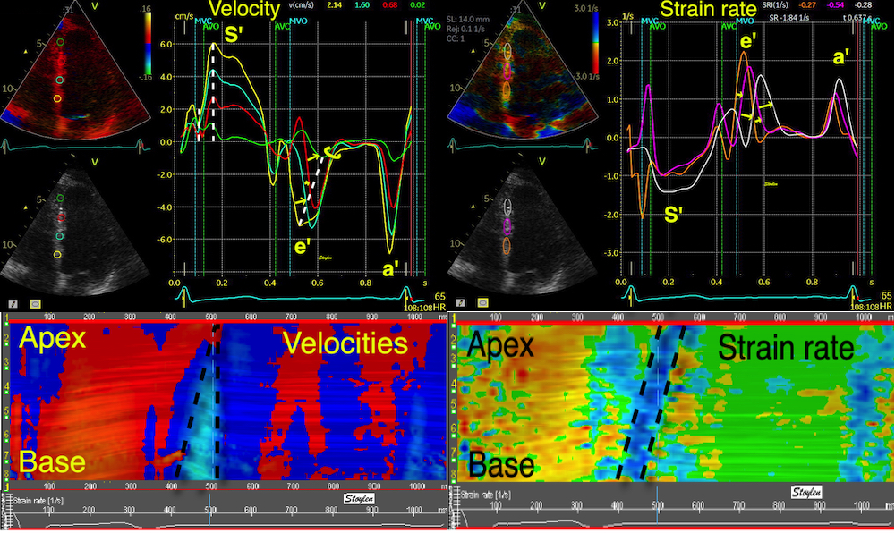
Left, velocities. The velocities of the e' sho0w a progressive delay of both start and peak from base to apex, while the ends are simultaneous. This is evident also from the triangular shape of the e' wave in the CAMM below left. In strain rate, the e' peaks show delay delay of both start, peak and end, from base to apex, as also seen by the elongation wave propagating from base to apex in the CAMM below right.

In the row of cars, the foremost car starts first, and then the second, third etc. the start proceeds as a wave backwards through the queue. The cyan colour colours the cars with changing distance between them, which is the last starting and the first still stationary, which is the place where deformation of the queue takes part.
 |
 |
| Tissue M-mode showing how the start point of the downward motion is at base, propagating towards the apex. | Diastolic strain rate propagation velocity can be measured as the slope of the elongation wave. |

Colouring the cars acquiring velocity in blue, we see the start of the wave in front, adding one car at a time till all have the same velocity, and thus are blue. Colouring only the cars with DIFFERENT velocity, we show the interval where distance increases, i.e. where the row deforms.


Elongation starts at the base, where the myocardium closest to the mitral ring is first that is free to move basally. This basal motion continues through the full early filling phase, and new myocardial tissue is added to the motion. The simultaneous elongation and thinning of the wall proceeds towards the apex as a discrete wave, but the elongated and thinned myocardium will still be moving.
The train rate propagation is reduced in reduced diastolic function (77). However, this is not a "new" finding, but relates to the finding of reduced e' in tissue Doppler.
 |
 |
| Relation between diastolic strain rate propagation of the E-wave and the peak early diastolic velocity of the annulus. If the wave propagates slower, the resulting velocity wave of the annulus will be broader and lower . | In reduced diastolic function as shown here to the right, there is a lower peak diastolic annular velocity as well as a reduced early magnitude of motion of the mitral ring. |
Strain rate propagation is thus a global measure that relates geometrically to the peak e' in tissue Doppler.
However, this also has consequences for measuring peak diastolic strain rate:
As already shown, the peaks of the locat strain rates are not simultaneous. This means that there is not "one" peak strain rate.

Diastolic strain rates are regional, showing different timing (delay) from base to apex. Processing strain rate for the whole wall will average them to one peak, but that peak will be very similar to the peak e' velocity of the mitral annulus, and it is doubtful whether it adds extra information.

We can se that the both the early and late filling are propagatoing from base to apex, and the mechanism for that is the same for both, as discussed here. However, tyhe propagation velocity differs, being higher in the a' wave than the e' wave (77).
| e' (cm/s) |
a' (cm/s) |
PVSe' (cm/s) |
PVSa' (cm/s) |
| 13.1 (2.8) | 10.2 (1.8) | 60 (12.9) | 94.0 (22.1) |
As the LV myocardium is under tension, although relaxing during the e', but being completely relaxed during the a' (at least in normal EDV), this is not surprising.
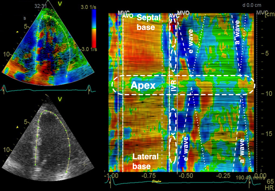
Curved M-mode showing the full M-mode from basal septum through the apex to the basal lateral wall. The isovolumic phases with apical lengthening and basal shortening is seen, as well as the propagation of the elongation waves both in early filling phase and during atrial systole, which also shows a propagation from base to apex, but with a higher propagation velocity. In addition, the elongation waves can be seen to either cross or return from the apex towards the base, but far weaker. This can also be seen above, as the basal strain rate are double peaked.
 |
 |
| CAMM and curves from
the septum, showing the complexity of the
diastolic strain rate with the different peaks
resulting from both elongation pre AVC, apical
elongation during IVR, elongation during early and
late filling, and return waves from apex,
resulting in double waves in the midwall and base. |
Curved M-mode
through the whole wall, showing how the elongation
waves look contiguous across the apex. |