TMM4175 Polymer Composites
Stress
The components of stress at a point are the forces per unit area acting on planes passing through the points. The tensor notation, or Einstein notation for stress is $\sigma_{ij}$ where $i,j=1,3,4$. The first index corresponds to the direction of the normal to the plane of interest and the second index corresponds to the direction of the force as illustrated in Figure-1 (left).
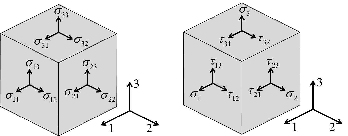
Figure-1: Components of stress in a 1,2,3 koordinate system
The stress tensor can be written as a 3 x 3 matrix:
\begin{equation} \boldsymbol{\sigma}= \begin{bmatrix} \sigma_{11} & \sigma_{21} & \sigma_{31} \\ \sigma_{12} & \sigma_{22} & \sigma_{32} \\ \sigma_{13} & \sigma_{23} & \sigma_{33} \end{bmatrix} \label{eq:stresstensor1} \tag{1} \end{equation}Force and moment equilibrium requires that the stress tensor to be symmetric (i.e., $\sigma_{ij}=\sigma_{ji}$). Furthmore, we will follow the common practice to use the notation $\tau_{ij}$ for shear stresses and use reduced notation for normal stresses (i.e., $\sigma_{ii}=\sigma_i$). Hence, the stresses by the simplified matrix notation becomes
\begin{equation} \boldsymbol{\sigma}= \begin{bmatrix} \sigma_{1} & \tau_{12} & \tau_{13} \\ \tau_{12} & \sigma_{2} & \tau_{23} \\ \tau_{13} & \tau_{23} & \sigma_{3} \end{bmatrix} \label{eq:stresstensor2} \tag{2} \end{equation}Due to the symmetry, there are only 6 independent components of stress.
In a coordinate system x,y,z as illustrated in Figure-2, the stress is written
\begin{equation} \boldsymbol{\sigma}= \begin{bmatrix} \sigma_{x} & \tau_{xy} & \tau_{xz} \\ \tau_{xy} & \sigma_{y} & \tau_{yz} \\ \tau_{xz} & \tau_{yz} & \sigma_{z} \end{bmatrix} \label{eq:stresstensor3} \tag{3} \end{equation}
Figure-2: Components of stress in a x,y,z coordinate system
If the concept of stress somehow gone under the radar during your materials and mechanical engineering studies, an introductory textbook on mechanics of materials, for example [1] will provide the proper background
Consider a stress state
$$ \boldsymbol{\sigma}= \begin{bmatrix} \sigma_{x} & \tau_{xy} & \tau_{xz} \\ \tau_{xy} & \sigma_{y} & \tau_{yz} \\ \tau_{xz} & \tau_{yz} & \sigma_{z} \end{bmatrix}= \begin{bmatrix} 100 & 20 & 0 \\ 20 & 50 & 0 \\ 0 & 0 & 0 \end{bmatrix} $$A straight forward NumPy-array representation is:
import numpy as np

S1=np.array ( [ [  100.0,  20.0,   0.0 ],
              [     20.0,  50.0,   0.0 ],
              [      0.0,   0.0,   0.0 ]  ])

I=np.identity(3)

print(  np.dot( (S1-I*110) , [1,0.2,0] ) )
The stress state above is an example of a plane stress case (stress exsists only on the 1-2 plane), while the two examples that follow are pure shear ($\tau_{yz} \ne 0$) and pure pressure ($\sigma_x=\sigma_y=\sigma_z=-P$) respectively:
S2=np.array ( [ [  0.0,   0.0,   0.0 ],
              [    0.0,   0.0,  50.0 ],
              [    0.0,  50.0,   0.0 ]  ])

S3=np.array ( [ [-20.0,   0.0,   0.0 ],
              [    0.0, -20.0,   0.0 ],
              [    0.0,   0.0, -20.0 ]  ])

print(S2)
print()
print(S3)
Eigenvalues and eigenvectors
The eigenvalues $\lambda$ and the eigenvectors $\mathbf{v}$ are the solutions of \begin{equation} (\boldsymbol{\sigma}-\mathbf{I}\lambda)\mathbf{v}=\mathbf{0} \label{eq:eigenv} \tag{4} \end{equation}
Plane stress example where $\sigma_z=\tau_{xz}=\tau_{yz}=0$ :
S1=np.array ( [ [  100.0,  20.0,   0.0 ],
              [     20.0,  50.0,   0.0 ],
              [      0.0,   0.0,   0.0 ]  ])

L,v = np.linalg.eig(S1)

print('Eigenvalues:')
print(L)
print()
print('Eigenvectors:')
print(v)
Note that the eigenvectors are the given by columns:
v1 = v[:,0]
v2 = v[:,1]
v3 = v[:,2]

print('The eigenvectors are:')
print()
print(v1, v2, v3)
Verify that equation (4) is true by computing \begin{equation} (\boldsymbol{\sigma}-\mathbf{I}\lambda)\mathbf{v} \tag{5} \end{equation}
I=np.identity(3)
print(  np.dot( (S1-I*L[0]) , v1 ) )
print()
print(  np.dot( (S1-I*L[1]) , v2 ) )
print()
print(  np.dot( (S1-I*L[2]) , v3 ) )
(except from some numerical noise: yes, all vectors are zero)
Pincipal stresses
The 1st, 2nd and 3rd principal stresses are found among the eigenvalues, where the 1st is the max value and the 3rd is the min value. That is:
s_1st = max(L)
s_3rd = min(L)

print('First principal stress =  ',s_1st)
print('Third principal stress =  ',s_3rd)
The directions of the principal stresses illustrated using matplotlib:
import matplotlib.pyplot as plt
%matplotlib inline
fig,ax = plt.subplots(figsize=(4,4))
ax.set_axis_off()
ax.set_xlim(-1.1,1.1)
ax.set_ylim(-1.1,1.1)

ax.arrow(0, 0, 1, 0.0, head_width=0.1, head_length=0.1, fc='black', ec='black')
ax.arrow(0, 0, 0.0, 1, head_width=0.1, head_length=0.1, fc='black', ec='black')
ax.text(0.9, 0.1, 'x')
ax.text(0.1, 0.9, 'y')

ax.arrow(0, 0, v1[0], v1[1], head_width=0.1, head_length=0.1, fc='red', ec='red')
ax.arrow(0, 0, v2[0], v2[1], head_width=0.1, head_length=0.1, fc='blue', ec='blue')

plt.show()

The angle between the 1st principal stress and the $x$ -axis is:
from math import degrees, acos
angle=degrees(acos(v1[0]))
print('{0:0.1f} degrees'.format(angle))
Maximum shear stress
The maximum shear stress is \begin{equation} \tau_{max}=\frac{1}{2}(\sigma_{max}-\sigma_{min}) = \frac{1}{2}(\sigma_{1st}-\sigma_{3rd}) \tag{6} \end{equation}
tau_max = (1/2)*(s_1st - s_3rd)
print('Maximum shear stress:',tau_max)
Isostatic, deviatoric and von Mises stress
The isostatic stress tensor $\boldsymbol{\sigma_0}$ is \begin{equation} \boldsymbol{\sigma_0}=\frac{1}{3}\big(\sigma_x+\sigma_y+\sigma_z\big)\mathbf{I} \tag{7} \end{equation}
iso=(1/3)*np.trace(S1)*np.identity((3))
print('Isostatic stress:\n\n',iso)
where the trace of $\boldsymbol{\sigma}$ is $\sigma_x+\sigma_y+\sigma_z$
print( np.trace(S1))
The deviatoric stress tensor, \begin{equation} \boldsymbol{\sigma_{dev}}=\boldsymbol{\sigma}-\boldsymbol{\sigma_0} \tag{8} \end{equation}
sdev=S1-iso
print('Deviatoric stress:\n\n',sdev)
The von Mises stress for a general state of stress is
\begin{equation} \sigma _{v}=\sqrt{\frac {1}{2}\big((\sigma_{x}-\sigma_{y})^{2}+(\sigma_{y}-\sigma_{z})^{2}+(\sigma_{z}-\sigma_{x})^{2}+6(\tau_{xy}^{2}+\tau_{yz}^{2}+\tau_{xz}^{2})\big)} \tag{9} \end{equation}or by the principal stresses:
\begin{equation} \sigma _{v}=\sqrt{\frac {1}{2}\big((\sigma_{1th}-\sigma_{2nd})^{2}+(\sigma_{2nd}-\sigma_{3rd})^{2}+(\sigma_{3rd}-\sigma_{1th})^{2}\big)} \tag{10} \end{equation}vonMises= ((1/2)*((L[0]-L[1])**2 + (L[0]-L[2])**2 + (L[1]-L[2])**2))**0.5
print('{0:0.4f}'.format(vonMises))
Alternatively:
vonMises=((3/2)*(np.sum(sdev**2)))**(1/2)
print('{0:0.4f}'.format(vonMises))
Python tips & tricks
The stress represented as a 3x3 matrix is quite often a sparse matrix. For instance, the matrix representation of a unidirectional stress has only one non-zero component and eight zeros. In such cases, modifying component(s) of an existing zero matrix requires less coding:
S4 = np.zeros((3,3))
S4[0,0]=100
print(S4)
S5 = np.zeros((3,3))
S5[1,2],S5[2,1]=50,50
print(S5)
A function with default values (and therefore the arguments are optional) can be a useful alternative:
def stressTensor(s1=0.0,s2=0.0,s3=0.0,s12=0.0,s13=0.0,s23=0.0):
    return np.array ( [ [s1 ,  s12,   s13 ],
                      [  s12,   s2,   s23 ],
                      [  s13,  s23,    s3 ]  ])

S6=stressTensor(s2=75)
S7=stressTensor(s13=60,s3=80)

print(S6)
print()
print(S7)
Assignment versus numpy.copy()
Remember that assignment statements in Python do not copy objects, and an array is a object in this sense. Hence, if a new variable is assigned to an existing variable pointing to an array as:
S8=S7
modifying a component of the new S8
S8[0,0]=99
will also modify S7 (or actually, S7 is still pointing to the same object):
S7
the numpy function numpy.copy() is similar to copy.deepcopy() for built-in mutable data types such as lists and dictionaries:
S9=np.copy(S7)
S9[1,1]=55

print(S9)
print()
print(S7)
Output formatting
Consider the following example with random numbers:
from random import random

S10 = stressTensor(s1=100*random(),s2=100*random(),s3=100*random(),s12=0.01*random())

print(S10)
The readability of this array is rather poor, and the precision is probably far beyond what is needed for any practial cases. Now, we may apply numpy.round():
print(np.round(S10,2))
The numpy.round() function is however not a formatting function but rather a operator returning a new array. A more proper and general approach is to use numpy.array2string() function:
print(np.array2string(S10, precision=2, suppress_small=True, separator=' ', floatmode='maxprec') )
References and further readings
- Hibbeler, R.C., and Kai Beng Yap. Mechanics of Materials. Harlow: Pearson, 2018.
- Herakovich, Carl T. Mechanics of Fibrous Composites. New York: Wiley, 1998.
- Daniel, Isaac M., and Ori Ishai. Engineering Mechanics of Composite Materials. 2nd ed. New York: Oxford University Press, 2006.
- Kollár, Lázló P., and George S. Springer. Mechanics of Composite Structures. Cambridge: Cambridge University Press, 2003.


Disclaimer:This site is about polymer composites, designed for educational purposes. Consumption and use of any sort & kind is solely at your own risk.
Fair use: I spent some time making all the pages, and even the figures and illustrations are my own creations. Obviously, you may steal whatever you find useful here, but please show decency and give some acknowledgment if or when copying. Thanks! Contact me: nils.p.vedvik@ntnu.no www.ntnu.edu/employees/nils.p.vedvik
Copyright 2021, All right reserved, I guess.