TMM4175 Polymer Composites

Home About Python Links Table of Contents

Shell elements and laminate theory¶

Figure-1 shows a shell based FEA model of a laminate subjected to a prescribed tensile strain in the $x$-direction imposed as displacements on the edges.

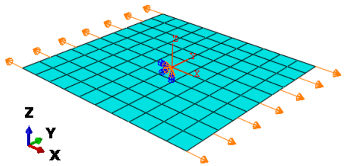
Figure-1: Laminate model

Dimensions: 100 x 100 x $h$, where the thickness $h$ is given by the section properties (layup)

Mesh: 10 x 10 elements of type S4R

Boundary conditions:

The node at origo is fixed for all DOF (both translations and rotations)
On the edge at $x$ = 50: $u_x$ = 0.5
On the edge at $x$ = -50: $u_x$ = -0.5

The boundary conditions for the node at origo will maintain the conditions: $w = 0$ and $\frac{\partial w}{\partial x}$ for $(x,y)$ = (0,0), see Laminate deformation.

The laminate midplane strain $\varepsilon_x^0$ becomes:

\begin{equation} \varepsilon_x^0 = \frac{\Delta u_x}{\Delta x} = \frac{0.5 -(-0.5)}{100}=0.01 \end{equation}

Example-1:¶

Consider a [0/90] laminate with the material, layup and loading as follows:

from laminatelib import laminateStiffnessMatrix, solveLaminateLoadCase, laminateThickness, layerResults
import numpy as np

m1={'E1':140000, 'E2':8000, 'v12':0.27, 'G12':5000,
    'XT':1000, 'YT':50, 'XC':800, 'YC':200, 'S12':50, 'S23':50, 'f12':-0.5}

layup1  =[ {'mat':m1 , 'ori':    0  , 'thi':1} , 
           {'mat':m1 , 'ori':   90  , 'thi':1}  ]

LSM1 = laminateStiffnessMatrix(layup1)

result = solveLaminateLoadCase(LSM1,ex=0.01)
N=result[0]
D=result[1]

print('Loads=',np.round(N,1))
print('Deformations=',np.round(D,6))

Loads= [598.3   0.    0.    0.    0.    0. ]
Deformations= [ 0.01     -0.000292 -0.        0.013378  0.       -0.      ]

Abaqus provides results for laminate loads and deformations as Section forces and moments and Section strains and curvatures. These must be specified in the Field Output Request for the step. The FEA results are:

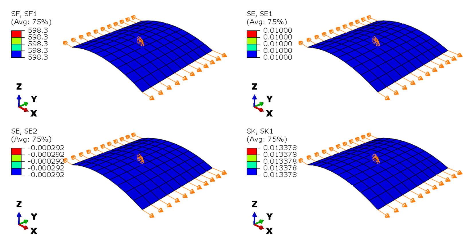
Figure-2: FEA-results: Laminate loads and deformations

The field output variables translate to:

SF1 = $N_x$
SE1 = $\varepsilon_x^0$
SE2 = $\varepsilon_y^0$
SK1 = $\kappa_x$

Out-of-plane displacement $u_z$ (=$w$) is:

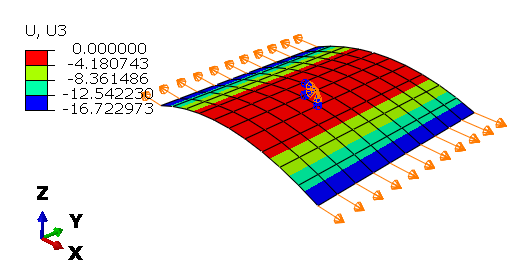
Figure-3: FEA-results: out-of-plane displacement

We can now compare the FEA results to the analytical displacement field derived in Laminate deformation:

\begin{equation} w(x,y) = -\frac{1}{2}\kappa_x x^2 -\frac{1}{2}\kappa_y y^2 -\frac{1}{2} \kappa_{xy} x y \end{equation}

For example, at $(x,y)$ = (50,50):

print( 'w=' , (- D[3]*50**2 - D[4]*50**2 - D[5]*50*50)/2  )

w= -16.722972972972975

3D-plot:

def illustrateCurvatures(Kx,Ky,Kxy):
    from mpl_toolkits.mplot3d import Axes3D
    import matplotlib.pyplot as plt
    %matplotlib inline
    from matplotlib import cm
    from matplotlib.ticker import LinearLocator, FormatStrFormatter
    import numpy as np
    fig = plt.figure(figsize=(8,4))
    ax = fig.gca(projection='3d')
    # Make data.
    X = np.linspace(-50, 50, 10)
    Y = np.linspace(-50, 50, 10)
    X, Y = np.meshgrid(X, Y)
    Z1 =  (- Kx*X**2 - Ky*Y**2 - Kxy*X*Y)/2
    surf1 = ax.plot_surface(X, Y, Z1, cmap=cm.coolwarm,
                        linewidth=0, antialiased=False)

illustrateCurvatures(D[3],D[4],D[5])

The stresses in the material coordinate system at the top of the last layer (layer-2) is:

layres=layerResults(layup=layup1,deformations=D)

print( layres[-1]['stress']['123']['top'] )

[ 9.67272625e+00  1.87176263e+02 -1.16566388e-14]

The corresponding FEA results are:

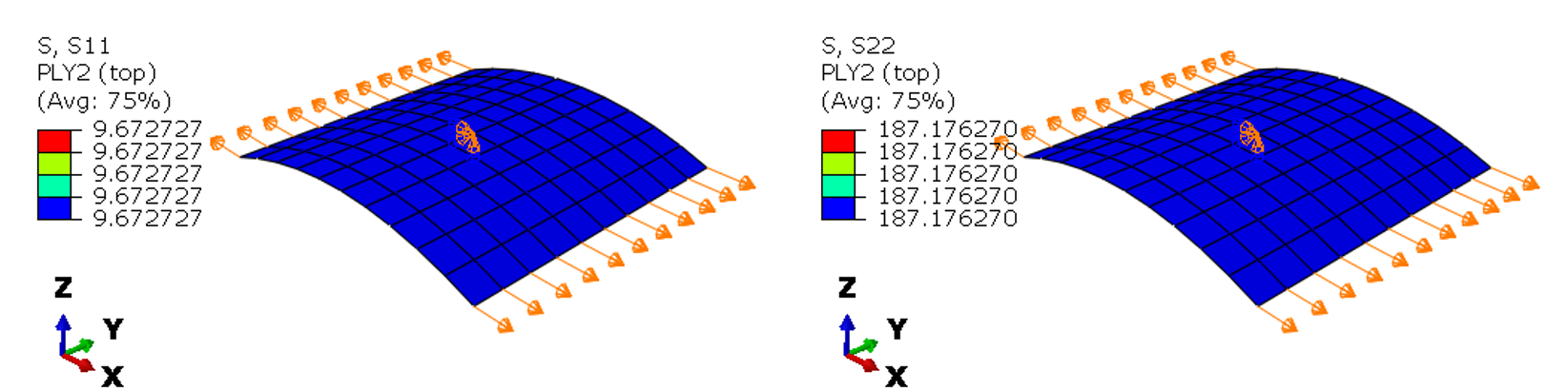
Figure-4: FEA-results: stresses

Example-2:¶

Consider a [-45/45] laminate with the material, layup and loading as follows:

m1={'E1':140000, 'E2':8000, 'v12':0.27, 'G12':5000,
    'XT':1000, 'YT':50, 'XC':800, 'YC':200, 'S12':50, 'S23':50, 'f12':-0.5}

layup1  =[ {'mat':m1 , 'ori':  -45  , 'thi':1} , 
           {'mat':m1 , 'ori':   45  , 'thi':1}  ]

LSM1 = laminateStiffnessMatrix(layup1)

result = solveLaminateLoadCase(LSM1,ex=0.01)
N=result[0]
D=result[1]

print('Loads=',np.round(N,1))
print('Deformations=',np.round(D,6))

Loads= [302.   0.   0.   0.   0.   0.]
Deformations= [ 0.01     -0.0051    0.        0.        0.       -0.006753]

Abaqus:

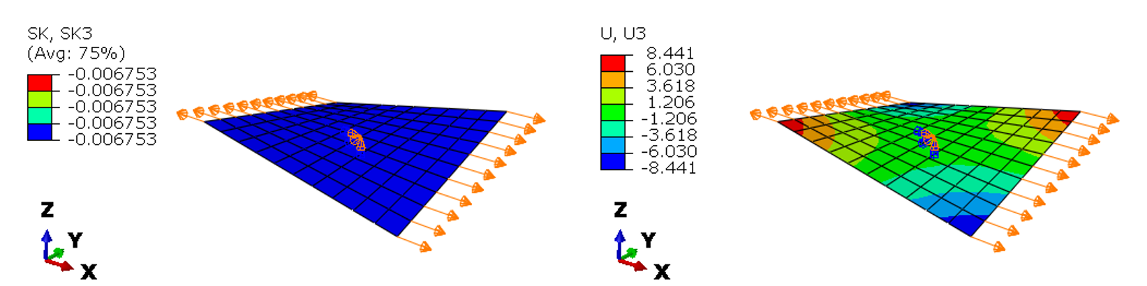
Figure-5: FEA-results: SK3 = $\kappa_{xy}$ and out-of-plane displacement

The out-of-plane displacement at the corner +$x$ and +$y$ is:

print( 'w=' , (- D[3]*50**2 - D[4]*50**2 - D[5]*50*50)/2  )

w= 8.441465264588228

illustrateCurvatures(D[3],D[4],D[5])

Summary¶

From abaqus documentation, with translation to laminate theory variables (...) as used in this course:

SF1: Direct membrane force per unit width in local 1-direction. ( $N_x$ )

SF2: Direct membrane force per unit width in local 2-direction. ( $N_y$ )

SF3: Shear membrane force per unit width in local 1–2 plane. ( $N_{xy}$ )

SF4: Transverse shear force per unit width in local 1-direction.

SF5: Transverse shear force per unit width in local 2-direction.

SF6: Thickness stress integrated over the element thickness.

SM1: Bending moment force per unit width about local 2-axis. ( $M_x$ )

SM2: Bending moment force per unit width about local 1-axis. ( $M_y$ )

SM3: Twisting moment force per unit width in local 1–2 plane. ( $M_{xy}$ )

SE1: Direct membrane strain in local 1-direction. ( $\varepsilon_x^0$ )

SE2: Direct membrane strain in local 2-direction. ( $\varepsilon_y^0$ )

SE3: Shear membrane strain in local 1–2 plane. ( $\gamma_{xy}^0$ )

SE4: Transverse shear strain in the local 1-direction.

SE5: Transverse shear strain in the local 2-direction.

SE6: Total strain in the thickness direction.

SK1: Curvature change about local 2-axis. ( $\kappa_x$ )

SK2: Curvature change about local 1-axis. ( $\kappa_y$ )

SK3: Surface twist in local 1–2 plane. ( $\kappa_{xy}$ )

Disclaimer:This site is about polymer composites, designed for educational purposes. Consumption and use of any sort & kind is solely at your own risk.
Fair use: I spent some time making all the pages, and even the figures and illustrations are my own creations. Obviously, you may steal whatever you find useful here, but please show decency and give some acknowledgment if or when copying. Thanks! Contact me: nils.p.vedvik@ntnu.no www.ntnu.edu/employees/nils.p.vedvik