TMM4175 Polymer Composites

Home About Python Links Table of Contents

Laminate deformation¶

The Kirchhoff assumption implies that the displacements at a position $z$ through the thickness are related to the midplane displacements and rotations expressed by:

\begin{equation} \begin{aligned} &u(x,y,z) = u_0(x,y)-z \frac{\partial w_0}{\partial x} \\ &v(x,y,z) = v_0(x,y)-z \frac{\partial w_0}{\partial y} \\ &w(x,y)=w_0(x,y) \end{aligned} \tag{1} \end{equation}

where $u$, $v$ and $w$ are the displacements in $x$, $y$ and $z$ directions respectively, and $u_0$, $v_0$ and $w_0$ are the displacements of the reference plane.

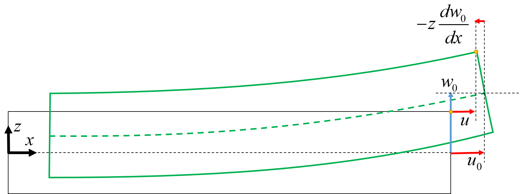
Figure-1: Kirchoff assumption

From the strain-displacement equations;

\begin{equation} \begin{aligned} &\varepsilon_x = \frac{\partial u}{\partial x} =\frac{\partial u_0}{\partial x} - z \frac{\partial^2 w_0}{\partial x^2} = \varepsilon_x^0 + z \kappa_x \\ &\varepsilon_y = \frac{\partial v}{\partial y} =\frac{\partial v_0}{\partial y} - z \frac{\partial^2 w_0}{\partial y^2} = \varepsilon_y^0 + z \kappa_y \\ &\gamma_{xy} = \frac{\partial u}{\partial y} + \frac{\partial v}{\partial x} =\frac{\partial u_0}{\partial y} + \frac{\partial v_0}{\partial x} - 2z \frac{\partial^2 w_0}{\partial x \partial y} = \gamma_{xy}^0 + z \kappa_{xy} \end{aligned} \tag{2} \end{equation}

where $\varepsilon_x^0$, $\varepsilon_y^0$ and $\gamma_{xy}^0$ are mid-plane strains and $\kappa_x$, $\kappa_y$ and $\kappa_{xy}$ are curvatures given by

\begin{equation} \kappa_x=-\frac{\partial^2 w}{\partial x^2}, \quad \kappa_y=-\frac{\partial^2 w}{\partial y^2}, \quad \kappa_{xy}=-2\frac{\partial^2 w}{\partial x \partial y} \tag{3} \end{equation}

The relations can now be summarized using matrix form as

\begin{equation} \begin{bmatrix} \varepsilon_x \\ \varepsilon_y \\ \gamma_{xy} \end{bmatrix}= \begin{bmatrix} \varepsilon_x^0 \\ \varepsilon_y^0 \\ \gamma_{xy}^0 \end{bmatrix}+z \begin{bmatrix} \kappa_x \\ \kappa_y \\ \kappa_{xy} \end{bmatrix} \tag{4} \end{equation}

or the short notation

\begin{equation} \boldsymbol{\varepsilon}' = \boldsymbol{\varepsilon}^0 + z \boldsymbol{\kappa} \tag{5} \end{equation}

Illustrating the curvatures:

The curvatures can be visualized by superposing the resulting out-of-plane displacement $w$ given by the contributions from $\kappa_x$, $\kappa_y$ and $\kappa_{xy}$:

$$ \frac{\partial^2 w}{\partial x^2} = -\kappa_x \Rightarrow \frac{\partial w}{\partial x} = -\kappa_x x + c_1 \Rightarrow w=-\frac{1}{2}\kappa_x x^2 + c_1 x + c_2 $$

The boundary conditions $w(x=0) = 0$ and $\frac{\partial}{\partial x}w(x=0)$ leads to

$$ w=-\frac{1}{2}\kappa_x x^2 $$

Correspondingly, the contribution from the curvature $\kappa_y$ when we assume that $\frac{\partial}{\partial y}w(x=0)$ is

$$ w=-\frac{1}{2}\kappa_y y^2 $$

For $\kappa_{xy}$:

$$ \frac{\partial^2 w}{\partial x \partial y} = -\frac{1}{2}\kappa_{xy} \Rightarrow \frac{\partial w}{\partial y} = -\frac{1}{2} \kappa_{xy} x + c_5 \Rightarrow w=-\frac{1}{2}\kappa_{xy} x y + c_5 y + c_4 $$

The boundary conditions $w(x=0) = 0$, $\frac{\partial}{\partial x}w(x=0)$ and $\frac{\partial}{\partial y}w(x=0)$ gives

$$ w=-\frac{1}{2}\kappa_{xy} x y $$

Finally;

\begin{equation} w(x,y) = -\frac{1}{2}\kappa_x x^2 -\frac{1}{2}\kappa_y y^2 -\frac{1}{2} \kappa_{xy} x y \tag{6} \end{equation}

Implementation and examples:

def illustrateCurvatures(Kx,Ky,Kxy):
    from mpl_toolkits.mplot3d import Axes3D
    import matplotlib.pyplot as plt
    from matplotlib import cm
    from matplotlib.ticker import LinearLocator, FormatStrFormatter
    import numpy as np
    fig = plt.figure(figsize=(6,4))
    ax = fig.gca(projection='3d')
    X = np.arange(-0.5, 0.6, 0.1)
    Y = np.arange(-0.5, 0.6, 0.1)
    X, Y = np.meshgrid(X, Y)
    Z1 =  (- Kx*X**2 - Ky*Y**2 - Kxy*X*Y)/2
    surf1 = ax.plot_surface(X, Y, Z1, cmap=cm.coolwarm, linewidth=0, antialiased=False)

%matplotlib inline
illustrateCurvatures(Kx=0.5, Ky=0.0, Kxy=0.0)

%matplotlib inline
illustrateCurvatures(Kx=-0.5, Ky=0.5, Kxy=0.0)

%matplotlib inline
illustrateCurvatures(Kx=0.0, Ky=0.0, Kxy=-0.25)

%matplotlib inline
illustrateCurvatures(Kx=0.0, Ky=0.25, Kxy=0.5)

Disclaimer:This site is about polymer composites, designed for educational purposes. Consumption and use of any sort & kind is solely at your own risk.
Fair use: I spent some time making all the pages, and even the figures and illustrations are my own creations. Obviously, you may steal whatever you find useful here, but please show decency and give some acknowledgment if or when copying. Thanks! Contact me: nils.p.vedvik@ntnu.no www.ntnu.edu/employees/nils.p.vedvik