TMM4175 Polymer Composites

Home About Python Links Table of Contents

Shear testing¶

There is a greater variety of shear test methods origin from the fact that it is difficult to obtaining a reasonably pure and uniform shear stress state in small and simple test specimen. Hence, many shear test methods actually involve a mixed mode loading which makes test results ambiguous with respect to true shear properties. Another problem is that some test methods adequately determine shear strength but not shear modulus and vice versa.

Tensile testing of symmetric [$\pm$45] laminates¶

Specimen

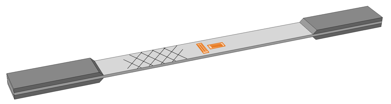
The shear modulus is derived from

\begin{equation} G_{12} = \frac{\overline{\sigma}_x}{2(\overline{\varepsilon}_x - \overline{\varepsilon}_y)} \tag{1} \end{equation}

where stresses and strains are the effective values in the laminate coordinate system.

Since this test method introduces all three in-plane stresses, the shear strength $S_{12}$ can be difficult to extract from the stress-strain data.

Example¶

A [45/-45/-45/45] laminate made of Carbon/Epoxy(a) material:

import matlib, laminatelib, plotlib
m = matlib.get('Carbon/Epoxy(a)')

layup=[{'mat': m, 'ori': 45, 'thi':1  },
       {'mat': m, 'ori':-45, 'thi':1  },
       {'mat': m, 'ori':-45, 'thi':1  },
       {'mat': m, 'ori': 45, 'thi':1  } ]

The shear strength and transverse tensile strength of this material is

print( 'Shear strength = ', m['S12'], 'MPa')
print( 'Transverse tensile strength = ', m['YT'], 'MPa')

Shear strength =  70 MPa
Transverse tensile strength =  40 MPa

An effective laminate stress $\overline{\sigma}_x = 140$ MPa corresponds to $|\tau_{12}|=70$ MPa since

\begin{equation} \tau_{12}=\frac{1}{2}(\sigma_{max}-\sigma_{min}) = \frac{1}{2}\overline{\sigma}_{xy} \tag{2} \end{equation}

From laminate theory:

sx = 140
Nx = sx*laminatelib.laminateThickness(layup)

ABD = laminatelib.laminateStiffnessMatrix(layup)
loads, defs = laminatelib.solveLaminateLoadCase(ABD, Nx=Nx)

ex, ey = defs[0], defs[1]
G12 = sx/(2*(ex-ey))

print('Computed G12=', round(G12), 'compared to material data:', m['G12'])

Computed G12= 4500 compared to material data: 4500

This method introduces not only shear stress but significant longitudinal and transverse stresses:

r = laminatelib.layerResults(layup,defs)

%matplotlib inline
plotlib.plotLayerStresses(r)

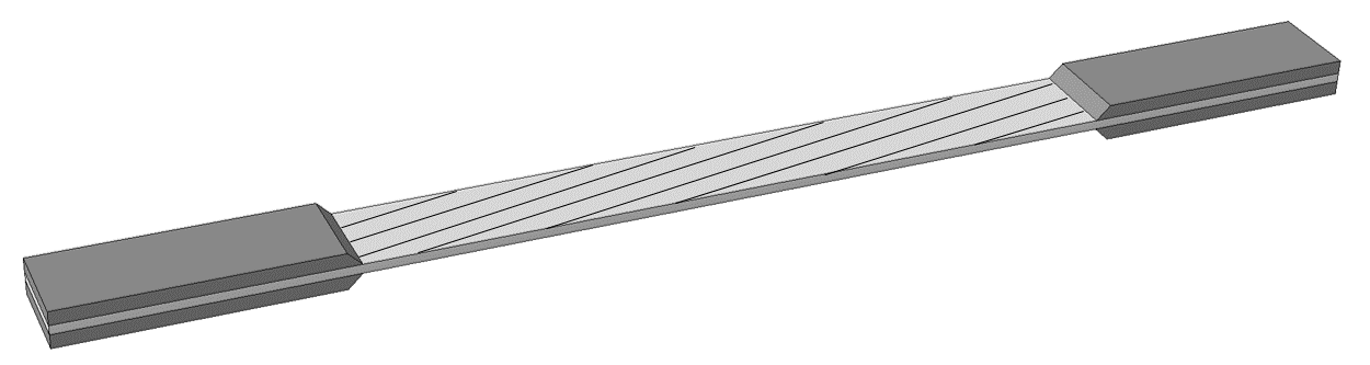
Off-axis tensile testing¶

The testing is conducted on unidirectional laminae where the fiber orientation is oriented by a relatively small angel (about 10 degrees) relatively to the loading direction.

Specimen

For idealized boundary conditions, the strains in the global system are:

\begin{equation} \begin{bmatrix} \varepsilon_x \\ \varepsilon_y \\ \gamma_{xy} \end{bmatrix}= \begin{bmatrix} S_{xx} & S_{xy} & S_{xs} \\ S_{xy} & S_{yy} & S_{ys} \\ S_{xs} & S_{ys} & S_{ss} \end{bmatrix} \begin{bmatrix} \sigma_x \\ 0 \\ 0 \end{bmatrix} \tag{3} \end{equation}

where $\sigma_x$ equals the tensile force divided by the cross section.

From the stresses and strains in the global system we compute the stresses and strains in the material coordinate system.

Example

Stresses as function of orientation angle for a loading corresponding to $\overline{\sigma}_x = 400$ MPa.

m = matlib.get('Carbon/Epoxy(a)')

plotlib.offAxisTest(m=m,sx=400,a=(0,35))

plotlib.offAxisTest(m=m,sx=400,a=(8,12))

Interpretation of the results shown in the graphs is left as exercise

Torque on thin-wall tubular hoop-wound specimen¶

This method enables an ideal uniform shear stress given by

\begin{equation} \tau_{12} = \frac{T}{2 \pi t R^2} \tag{4} \end{equation}

where $T$ is the torque, $t$ is the wall thickness and $R$ is the radius of the tube.

Disclaimer:This site is about polymer composites, designed for educational purposes. Consumption and use of any sort & kind is solely at your own risk.
Fair use: I spent some time making all the pages, and even the figures and illustrations are my own creations. Obviously, you may steal whatever you find useful here, but please show decency and give some acknowledgment if or when copying. Thanks! Contact me: nils.p.vedvik@ntnu.no www.ntnu.edu/employees/nils.p.vedvik