Grating lobes
In this module we will define what grating lobes are, and we will investigate how the distance between consective elements, often referred to as array pitch, can be optimised to improve imaging quality.
Related material:
Stefano Fiorentini <stefano.fiorentini@ntnu.no>
Last edit 3-10-2020
Array pitch
Once all of the layers are glued together, we have a monolithic ultrasound transducer. It cannot be used for ultrasound imaging yet, since it lacks the independent elements needed for electronic focusing and steering. An array transducer is obtained by dicing a monolithic transducer into evenly-sized elements. The space between elements is referred to as kerf. Generally speaking, the kerf should be as small as possibile to maximise the transducer element surface. However, some space is needed between consecutive elements to ensure that they can move independently. The distance between consecutive element centers is referred to as array pitch. Knowing element size \(d\) and kerf \(k\), the array pitch can be derived as
given a fixed aperture size \(a\), an estimate of the number of elements is given by
Grating lobes
In the next examples we are going investigate the effect of the array pitch on the ultrasound beam. We are going to simulate a probe with 3 MHz center frequency, 2 cm aperture size, and 10 μm kerf. The transducer is focused at 4 cm depth, without steering. The ultrasound beam propagates in a medium with speed of sound \(c_0 = 1540\) m/s. We are going to simulate two values for the array pitch, \(p = \lambda\) and \(p = 2\lambda\). Since kerf and aperture size are fixed, a different array pitch will result in different element size and number of elements. Solve the Raleigh integral numerically to simulate the ultrasound beam given the two transducer configurations.
% Transducer and medium properties
f0 = 3e6;                                   % pulse frequency [MHz]
rho = 1020;                                 % medium density [kg/m3]
c0 = 1540;                                  % medium speed of sound [m/s]
lambda = c0/f0;                             % wavelength [m]
w0 = 2*pi*f0;                               % angular frequency [rad/s]
k = w0/c0;                                  % wavenumber [rad/m]
a = 2e-2;                                   % transducer width [m]
b = 5e-3;                                   % transducer height [m]
focus = [0, 0, 4e-2];                       % focus position [m]
v0 = 1e-3;                                  % surface velocity [m/s]
pitch = [lambda, 2*lambda];                 % array pitch
kerf =  10e-6;                              % kerf [m]
element_size = pitch - kerf;                % element size [m]
N_elements = round((a-kerf)./pitch);        % number of elements [adim]

% Simulation parameters
N = 5e2;                                    % number of monte-carlo sources

az = linspace(-pi/4, pi/4, 256);
r = linspace(0, 6e-2, 256);
[AZ, R] = ndgrid(az, r);
[Z, X] = pol2cart(AZ, R);

N_pixels = numel(X);

figure('Color', 'w')

for p = 1:length(pitch)
    % initialise pixel map
    map = zeros(1, N_pixels);

    % calculate position of element center
    element_center = (1:N_elements(p))*pitch(p);
    element_center = element_center - mean(element_center);

    for n = 1:N_elements(p)
        fprintf(1, 'Computing element %d of %d\n', n, N_elements(p));

        % We set random source location within the element surface
        s = [random('unif', -element_size(p)/2, element_size(p)/2, [N, 1]), ...
            random('unif', -b/2, b/2, [N, 1]), ...
            zeros([N,1])] + [element_center(n), 0, 0];

        % Compute distance from all sources to all pixels
        R = sqrt( (s(:,1) - X(:).').^2 + ...
            s(:, 2).^2 + ...
            (s(:, 3) - Z(:).').^2);

        % Compute the focusing distance difference
        Rf = sqrt(sum(([element_center(n), 0, 0]-focus).^2, 2))-sqrt(sum(focus.^2));

        % Compute Green function
        green = exp(1i*k*Rf) .* exp(-1i*k*R)./(2*pi*R);

        % We add the contribution from all sources
        map =  map + sum(green, 1);
    end

    % Calculate pressure field
    map = 1j*w0*rho*v0*map;

    % Reshape results;
    map = reshape(map, size(X));

    % Apply log compression
    map = 20*log10(abs(map) / max(abs(map(:))));

    % Plot
    subplot(1,length(pitch),p)
    surface(X*1e3, Z*1e3, map, 'LineStyle', 'none')
    box on
    grid on;
    set(gca, 'YDir', 'reverse', 'Layer', 'top')
    colorbar
    caxis([-40 0])
    axis equal tight
    xlabel('x [mm]')
    ylabel('z [mm]')
    title('SPL [dB]')
end

The transducer with larger pitch exhibits spurious beams, which are oriented away from the focal point. These beams are referred to as grating lobes and are a major source of artifacts in ultrasound imaging. As shown in the examples, a pitch equal to the wavelength λ is sufficient to avoid grating lobes. Since ultrasound imaging is based on wide-band pulses, the pitch must be designed so that grating lobes are avoided at the maximum operating frequency of the transducer. Moreover, in the previous example we have not considered beam steering. What happens in this case?
% Transducer and medium properties
f0 = 3e6;                                   % pulse frequency [MHz]
rho = 1020;                                 % medium density [kg/m3]
c0 = 1540;                                  % medium speed of sound [m/s]
lambda = c0/f0;                             % wavelength [m]
w0 = 2*pi*f0;                               % angular frequency [rad/s]
k = w0/c0;                                  % wavenumber [rad/m]
a = 2e-2;                                   % transducer width [m]
b = 5e-3;                                   % transducer height [m]
focus = [2e-2, 0, 4e-2];                    % focus position [m]
v0 = 1e-3;                                  % surface velocity [m/s]
pitch = [lambda/2, lambda];                 % array pitch
kerf =  10e-6;                              % kerf [m]
element_size = pitch - kerf;                % element size [m]
N_elements = round((a-kerf)./pitch);        % number of elements [adim]

% Simulation parameters
N = 5e2;                                    % number of monte-carlo sources

az = linspace(-pi/4, pi/4, 256);
r = linspace(0, 6e-2, 256);
[AZ, R] = ndgrid(az, r);
[Z, X] = pol2cart(AZ, R);

N_pixels = numel(X);

figure('Color', 'w')

for p = 1:length(pitch)
    % initialise pixel map
    map = zeros(1, N_pixels);

    % calculate position of element center
    element_center = (1:N_elements(p))*pitch(p);
    element_center = element_center - mean(element_center);

    for n = 1:N_elements(p)
        fprintf(1, 'Computing element %d of %d\n', n, N_elements(p));

        % We set random source location within the element surface
        s = [random('unif', -element_size(p)/2, element_size(p)/2, [N, 1]), ...
            random('unif', -b/2, b/2, [N, 1]), ...
            zeros([N,1])] + [element_center(n), 0, 0];

        % Compute distance from all sources to all pixels
        R = sqrt( (s(:,1) - X(:).').^2 + ...
            s(:, 2).^2 + ...
            (s(:, 3) - Z(:).').^2);

        % Compute the focusing distance difference
        Rf = sqrt(sum(([element_center(n), 0, 0]-focus).^2, 2))-sqrt(sum(focus.^2));

        % Compute Green function
        green = exp(1i*k*Rf) .* exp(-1i*k*R)./(2*pi*R);

        % We add the contribution from all sources
        map =  map + sum(green, 1);
    end

    % Calculate pressure field
    map = 1j*w0*rho*v0*map;

    % Reshape results;
    map = reshape(map, size(X));

    % Apply log compression
    map = 20*log10(abs(map) / max(abs(map(:))));

    % Plot
    subplot(1,length(pitch),p)
    surface(X*1e3, Z*1e3, map, 'LineStyle', 'none')
    box on
    grid on;
    set(gca, 'YDir', 'reverse', 'Layer', 'top')
    colorbar
    caxis([-40 0])
    axis equal tight
    xlabel('x [mm]')
    ylabel('z [mm]')
    title('SPL [dB]')
end
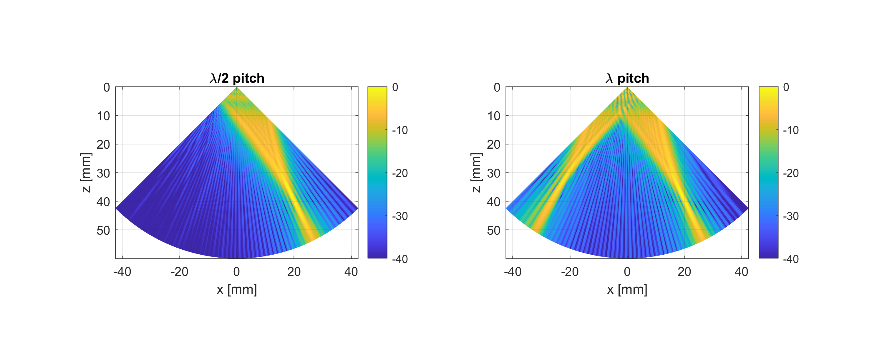
An array pitch equal to λ/2 guarantees the absence of grating lobes under any focusing and steering condition. So why not design any probe with λ/2 pitch? One reason lies in the total number of elements that a transducer would have. Let’s consider a typical probe used in linear imaging, with 4 cm aperture, 10 μm kerf, 7 MHz center frequency and 100% relative bandwidth. Calculate the number of elements that the transducer would have if the pitch were λ/2 and λ
f0 = 8e6;                                 % transducer center frequency [MHz]
df = 1;                                     % relative bandwidth [adim]
c0 = 1540;                                  % medium speed of sound [m/s]
a = 2e-2;                                   % transducer width [m]
kerf =  10e-6;                              % kerf [m]

fmax = f0 + f0*df/2;                        % transducer max operating frequency
lambda = c0/fmax;                           % wavelength [m]

pitch = [lambda/2, lambda];                 % array pitch

N_elements = round((a-kerf)./pitch);        % number of elements [adim]

fprintf(1, ['The total number of elements is %d for λ/2 pitch ', ...
    'and %d for λ pitch.\n'], N_elements(1), N_elements(2))
The total number of elements is 312 for λ/2 pitch and 156 for λ pitch.
Designing a linear probe with λ/2 pitch would require a very high number of elements. However, a commercial ultrasound scanner can generally operate a maximum of 256 elements only. For this reason, linear probes are designed with pitch close to λ and are used in combination with linear scans, so that the ultrasound beam is not steered.