TMM4175 Polymer Composites

Home About Python Links Table of Contents

Viscoelastic behavior¶

The term Viscoelasticity suggests a mechanical behaviour that is partly viscous and partly elastic. A viscous material exhibits time-dependent behavior when a stress is applied, while an elastic material deforms instantaneously when subjected to a load. A viscous deformation is generally a permanent deformation, while elastic deformation implies that the material returns to the original configuration when the load is removed.

Polymers are characterized by the fact that their behavior under load or deformation is, to a large extent, time dependent even at room temperature. Moreover, their response to a load or deformation will depend, in some cases, upon any previous load, deformation or temperature history. Two simple modes of viscoelastic manifestation is creep and relaxation

Creep and relaxation¶

Creep is the the time-dependent deformation under a constant load as illustrated in Figure-1 a).

When assuming linear viscoelasticity, the creep compliance $D(t)$ is expressed as

\begin{equation} D(t)=\frac{\varepsilon(t)}{\sigma}, \quad \sigma= \begin{cases} 0 & \quad t<0\\ \sigma_0 & \quad t \ge 0 \end{cases} \tag{1} \end{equation}

Relaxation is the gradual decrease in stress under a constant deformation as illustrated in Figure-1 b).

The relaxation modulus $E(t)$ is expressed as

\begin{equation} E(t)=\frac{\sigma(t)}{\varepsilon}, \quad \varepsilon= \begin{cases} 0 & \quad t<0\\ \varepsilon_0 & \quad t \ge 0 \end{cases} \tag{2} \end{equation}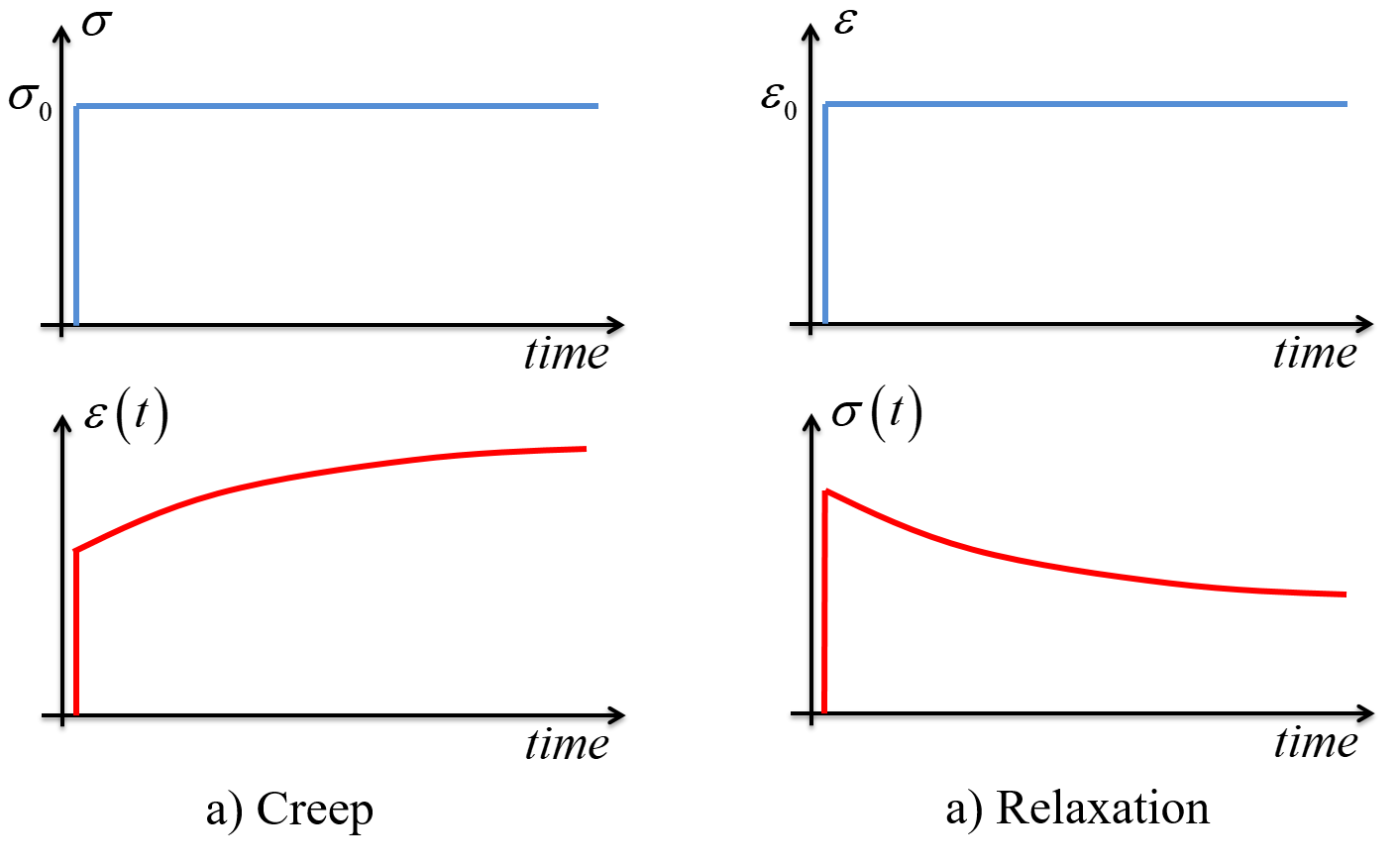

Figure-1: Creep and relaxation

Linear versus non-linear viscoelasticity¶

Linear viscoelasticity implies that the creep compliance $D(t)$ and the relaxation modulus $E(t)$ are not dependent on the stress and/or strain magnitudes. That is:

\begin{equation} E(t)=\frac{\sigma_1(t)}{\varepsilon_1}=\frac{\sigma_2(t)}{\varepsilon_2}=\frac{\sigma_3(t)}{\varepsilon_3}... \tag{3} \end{equation}

where $\varepsilon_i$ are different magnitudes of constant strains applied at $t=0$ and $\sigma_i(t)$ are the corresponding time-dependent stresses. Hence, the relaxation modulus $E(t)$ has time $t$ as the only variable.

The assumption of linear viscoelasticity should be evaluated carefully: The assumption is reasonably valid for small strains for many polymers, but becomes more inaccurate for larger strains. The concept of linear viscoelasticity is however very useful due to the simplified material models and superpositions that can be derived and performed from this assumption.

While a linear viscoelastic reponse of stress for an imposed instantaneous strain is simply $\sigma(t) = E(t)\varepsilon_0$, a nonlinear viscoelastic response would generally require that the state of stress and strain are included, i.e., $\sigma(t) = E(t,\sigma, \varepsilon_0)\varepsilon_0$.

Prony series¶

Creep compliance and relaxation modulus for linear viscoelastic materials are generally described by Prony series.

The creep compliance has the form

\begin{equation} D(t) = D_{\infty} - \sum_{i=1}^n D_i \exp(-t/\tau_i) \tag{4} \end{equation}

where $D_{\infty}$ is the apparent compliance at infinite time, and $\tau_i$ are called time constants.

Equation (4) can alternatively be expressed by

\begin{equation} D(t) = D_{0} + \sum_{i=1}^n D_i\big(1- \exp(-t/\tau_i)\big) \tag{5} \end{equation}

where $D_0$ is the instantaneous compliance at time $t=0$.

Example:

import numpy as np
import matplotlib.pyplot as plt
%matplotlib inline

D0= 1.0  # Compliance at t=0
n = 5    # number of terms in the summation
    
Di=(0.2,  0.3,  0.3,  0.2, 0.1)  # Compliance components in the summation
Ti=(2,  10,  50,  200, 800)      # time constants (tau)
    
t_lin=np.linspace(start= 0,stop=1000,num=100)  # a linear list from 0 to 1000
t_log=np.logspace(start=-1,stop=3.0,num=100)   # a logarithmic list from 0 to 1000
    
Dt_lin=D0  # initial value before summation
Dt_log=D0  # initial value before summation
    
for i in range(0,n):
    Dt_lin = Dt_lin + Di[i]*(1-np.exp(-t_lin/Ti[i]))
    Dt_log = Dt_log + Di[i]*(1-np.exp(-t_log/Ti[i]))   
    
# Plot with linear time axis:

fig,(ax1,ax2)=plt.subplots(nrows=2,ncols=1,figsize=(8,8))    
ax1.plot(t_lin,Dt_lin,label='Creep compliance')
ax1.set_xlim(0, )
ax1.set_ylim(0, )
ax1.set_xlabel('time')
ax1.set_ylabel('D(t)')
ax1.set_title('Creep, linear time scale')
ax1.legend(loc='lower right')
ax1.grid(True)

# Plot with logarithmic time axis

ax2.semilogx(t_log,Dt_log,label='Creep compliance')
ax2.set_xlim(0.1, )
ax2.set_ylim(0, )
ax2.set_xlabel('time')
ax2.set_ylabel('D(t)')
ax2.set_title('Creep, logarithmic time scale')
ax2.legend(loc='lower right')
ax2.grid(True)

plt.tight_layout()
plt.show()

The relaxation modulus has the form

\begin{equation} E(t) = E_{0} - \sum_{i=1}^n E_i\big(1- \exp(-t/\tau_i)\big) \tag{6} \end{equation}

where $E_0$ is the instantaneous modulus at time $t=0$.

If the polymer matrix behaves in a viscoelastic manner, what is the consequences regarding the properties and behavior of the fiber composite?

Disclaimer:This site is about polymer composites, designed for educational purposes. Consumption and use of any sort & kind is solely at your own risk.
Fair use: I spent some time making all the pages, and even the figures and illustrations are my own creations. Obviously, you may steal whatever you find useful here, but please show decency and give some acknowledgment if or when copying. Thanks! Contact me: nils.p.vedvik@ntnu.no www.ntnu.edu/employees/nils.p.vedvik